1. Introduction

Kinodynamic motion planning is essential in robotics, addressing the challenge of navigating dynamic environments while respecting both kinematic and dy- namic constraints. This field underpins the development of autonomous sys- tems, from self-driving vehicles to robots in varied settings, emphasizing the

need for algorithms that can manage movement feasibility, dynamic limitations, and environmental interactions effectively.

Among the strategies, tree sampling-based planners like RRT, RRT*, and DIRT stand out for their use of stochastic sampling to balance exploration and exploitation of the state space. This study focuses on comparing these plan- ners, especially highlighting the benefits of integrating learned controls—control strategies augmented by machine learning—to enhance their efficiency.

By examining the performance of these algorithms with and without learned controls, my research aims to shed light on their relative strengths and limita- tions, contributing insights to the advancement of motion planning in complex and dynamic environments.

2. Literature Review

Kinodynamic motion planning is at the forefront of robotics research, blending kinematic constraints with dynamic capabilities to navigate through intricate environments. The advent of tree-based algorithms such as RRT, RRT*, and DIRT has markedly enhanced the adaptability and efficiency of autonomous systems.

Introduced by LaValle and Kuffner [9], the Rapidly-exploring Random Tree (RRT) algorithm was a significant leap forward, efficiently covering high-dimensional spaces. This innovation paved the way for RRT* by Karaman and Frazzoli [8], which optimized the original by guaranteeing asymptotic optimality. The Dom- inance Informed Region Trees (DIRT) concept, developed by Littlefield and Bekris [10], further advanced kinodynamic planning by utilizing dominance re- gions to guide sampling decisions.

The fusion of traditional algorithms with intelligent controls, particularly through machine learning, has opened new horizons in autonomous navigation. Pan et al. [2] demonstrated the potential of integrating sampling-based algo- rithms with machine learning to improve motion planning. This approach is further exemplified by the work of Na Lin, Lu Bai, and Ammar Hawbani [4] in cooperative multi-agent path planning, and by Raihan Islam Arnob and Gre- gory J. Stein [6] in navigating partially-mapped environments, emphasizing the value of computational intelligence in addressing navigation challenges.

Janson and Pavone [7] highlighted the transformative potential of machine learning in enhancing pathfinding algorithms for real-time scenarios, paving the way for the incorporation of Deep Reinforcement Learning (DRL) into motion planning. The groundbreaking work by Silver et al. [1] on DRL demonstrates its capacity to enable systems to adapt to changing environments efficiently.

This review situates my research within a vibrant field, exploring the effi- cacy of algorithms like RRT, RRT*, and DIRT under dynamic conditions. By weaving together these threads of inquiry, we aim to further the discourse on kinodynamic motion planning, enriching the pool of strategies for enhancing autonomous navigation through computational and learned controls.

3. Methodology

This section delves into the methodologies employed to implement, evaluate, and compare the kinodynamic motion planning algorithms: RRT-Uninformed (RRT-U), RRT-Fully Informed (RRT-FI), RRT*, and Dominance Informed Re- gion Trees (DIRT).I detail the algorithmic foundations, evaluation metrics, and the experimental setup used in our comparative analysis.

3.1. RRT-Uninformed & RRT-Fully Informed

In this subsection, I present a unified RRT framework that encapsulates the strategies of both RRT-Uninformed (RRT-U) and RRT-Fully Informed (RRT- FI). By introducing a parameter α, the algorithm seamlessly toggles between RRT-U’s stochastic exploration and RRT-FI’s goal-directed search. This ap- proach allows for an adaptable exploration strategy, efficiently bridging the two variants and illustrating their applicability across different scenarios within a singular, cohesive algorithm.

The unified RRT algorithm operates as follows:

1. Initialize the tree with a node x_init.

2. Define α based on strategy: 0 for RRT-U, 1 for RRT-FI.

3. While the goal is not achieved:

If α = 0, sample a random point x_rand using the RRT-U strategy.

Else, sample towards the goal x_goal as per the RRT-FI strategy.

Find the nearest node x_near in the tree to x_rand.

Steer from xnear towards xrand to generate a new node xnew.

If xnew is valid, add it to the tree.

3.2. Rapidly-Exploring Random Tree Star (RRT*)

As an extension, RRT* incorporates a path optimization mechanism, reassessing and restructuring the tree to enhance path quality through cost minimization. This iterative refinement process is pivotal for achieving an optimal solution over time.

The RRT* algorithm procedure is as follows:

1. Initialize the tree with x_init.

2. While not at the goal:

Sample a random point x_rand.

Find the nearest node x_near in the tree to x_rand.

Steer from x_near towards x_rand to generate a new node x_new.

If x_new is valid, insert it into the tree and attempt to rewire the tree in the vicinity of x_new.

3.3. DIRT

The decision-making in DIRT is based on evaluating potential controls to apply at each node. For a given node x, the set of possible controls U is evaluated based on the cost function J which takes into account the distance to the goal d(x, x_goal) and the heuristic information h(x):

J (x, u) = α · d(f (x, u), x_goal) + β · h(f (x, u))

where f (x, u) represents the state transition function applying control u at state x, α and β are weighting parameters, and h(x) is the heuristic value of state x.

3.4. Metrics

The performance evaluation of the algorithms was based on a set of quantitative metrics, each designed to assess different aspects of efficiency and effectiveness in pathfinding. These metrics are crucial for understanding the algorithms’ capabilities in navigating complex environments.

Success Rate: The success rate is a critical indicator of reliability, reflecting the proportion of trials where the algorithm successfully identifies a viable path to the goal. It is mathematically represented as:

\( Success Rate=\frac{Number of Successful Trials}{Total Number of Trials} \) (1)

This metric is pivotal for evaluating the algorithm’s ability to consistently find solutions across a wide range of scenarios.

Iterations: This metric measures the computational effort required by the algorithm, quantifying the average iterations needed to discover the first valid path. It is computed using the formula:

\( Iterations=\frac{\sum Iterations per Trial}{Total Number Trials} \)

(2)

A lower average signifies greater efficiency, indicating that the algorithm requires fewer steps to reach a solution.

Path Cost: The total cost of the path, denoted as C_path, is defined by the cumulative distances between consecutive nodes along the path, calculated as follows:

\( {C_{path}}=\sum _{i=1}^{N-1}d({n_{i}},{n_{i+1}}) \) (3)

Here, N is the total number of nodes in the path, d represents the distance between consecutive nodes, and n_i and n_i+1 are sequential nodes along the path. The path cost is an essential measure of the solution’s quality, with lower costs indicating more efficient paths.

These metrics collectively provide a comprehensive framework for assessing the performance of pathfinding algorithms, offering insights into their efficiency,

effectiveness, and the quality of the solutions they generate. Revising your section with more detail on the generated grid environments, we can elaborate on the configurations, obstacles, and rationale behind the transition from the initial to the refined setup. This enhancement will not only clarify the experimental conditions but also underline the progression and decision-making process in adapting the setup for improved pathfinding evaluation.

3.5. Experimental Setup

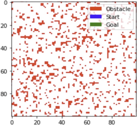
My journey commenced with an experimental setup featuring a grid populated with square blocks randomly designated as obstacles, chosen to present a sim- plified yet challenging landscape for pathfinding algorithms. This setup tested the algorithms’ capability to navigate through environments where obstacles completely block paths, necessitating the exploration of alternative routes. De- spite its initial utility, this binary obstacle model introduced complexities that detracted from my primary research goals, overemphasizing exhaustive search tactics over nuanced navigation strategies.

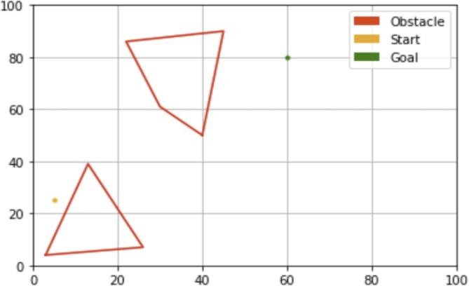
Influenced by Jiang’s research on complex obstacle navigation[3] and Cui’s research on optimized sampling point[5], I refined my setup by integrating polyg- onal obstacles within a versatile grid, better reflecting the varied shapes found in both natural and urban terrains. The adoption of floating-point nodes en- hanced my model’s precision, enabling the identification of more direct and efficient paths. Moreover, I conceptualized the destination not as a pinpointed location but as a broader target area, aligning with real-world scenarios where reaching a vicinity is often the objective. This adaptation allowed my Rapidly- exploring Random Trees (RRT) algorithms to recognize any node within this area as a successful end, introducing a flexible approach to path completion.

This progression from a simplistic binary model to a comprehensive, realistic framework marked a pivotal advancement in my research. It not only enabled a deeper evaluation of pathfinding algorithms but also ensured my methodologies resonated with the intricate demands of real-world navigation, establishing a solid foundation for future exploration in the field.

4. Results

The evaluation of the planning algorithms—DIRT, RRT-FI (Fully Informed), RRT-U (Uninformed), and RRT*—was conducted based on their success rates, the number of iterations to achieve the first solution, and the path costs of both the first and final solutions. This comprehensive assessment was carried out over 50 randomly generated grid environments, ensuring consistency in parameters such as vision radius, edge increment, and edge length across all tests.

4.1. Results Visualization

To visualize the results we obtained, we selected representative examples of each of the implemented algorithms run on the same grid.

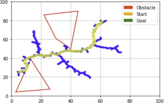
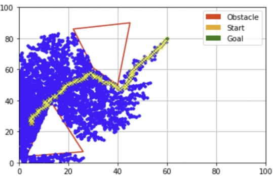
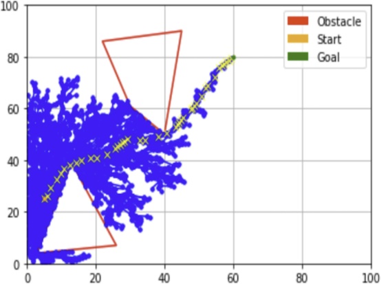
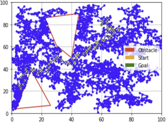
My comparative analysis of pathfinding algorithms—Fully Informed RRT, Uninformed RRT, RRT*, and DIRT highlights distinct efficiencies and path qualities, primarily influenced by the availability of environmental information. Fully Informed RRT in Figure3 excels in well-informed settings, producing opti- mal paths with minimal exploration. figure 5 demonstrates the efficiency of the path refinement approach. In contrast, DIRT in Figure 6 and Uninformed RRT

in Figure 4 require additional iterations but offer flexibility in unpredictable environments.

Notably, DIRT emerges as a balanced solution, leveraging the strengths of RRT* by offering a middle ground in terms of computational demand and ex- ploration depth. These insights highlight the importance of algorithm selection based on the specific needs of the operational environment, guiding strategic algorithm deployment in diverse settings and informing future developments in pathfinding technology.

4.2. Comparative Evaluation of Algorithm Performance

The core evaluation metrics—Success Rate, Number of Iterations, and Path Cost—serve as benchmarks for assessing each algorithm’s performance. Table 1 consolidates these metrics, facilitating a comprehensive analysis.

Table 1. Average Results of Planning Algorithms Evaluation

*FI = Fully Informed, U = Uninformed

The Success Rate (Equation 1), defined as the proportion of trials in which the algorithm successfully identifies a viable path from the starting point to the goal, serves as a primary indicator of reliability. The Number of Iterations (Equation 2) and the Path Cost (Equation 3) further provide insights into the computational efficiency and solution optimality, respectively.

The analysis reveals RRT-FI and DIRT achieving a 100% success rate, indi- cating their high reliability in pathfinding. Notably, DIRT’s approach—continuing exploration beyond the initial solution—manifests in its unique balance between exploration depth and computational efficiency, as evidenced by its iterations and path cost metrics.

This juxtaposition of algorithmic performance highlights the critical impor- tance of selecting an appropriate pathfinding algorithm based on the specific requirements and constraints of the operational environment. The insights de- rived from this comparative study not only inform the strategic deployment of algorithms but also provide valuable directions for future research and develop- ment in the field of pathfinding technology.

5. Discussion

The comparative evaluation of the planning algorithms: DIRT, RRT-FI, RRT- U, and RRT*—provides significant insights into their performance in terms of success rate, iterations to achieve the first solution, and path costs for both

initial and refined solutions. The results, drawn from 50 randomly generated grid environments, underscore the nuanced efficacy and optimization potential inherent in each algorithm under consistent conditions.

5.1. Algorithm Performance and Optimization

DIRT’s standout performance, characterized by a 100% success rate and the unique capability to iteratively refine the path cost, underscores its robustness and efficiency. This iterative refinement, absent in the RRT variants, highlights DIRT’s superior optimization over time, making it particularly suitable for ap- plications where gradual improvement of the solution is feasible and desirable. On the other hand, the observation that RRT-FI, despite its fully informed nature, does not always secure the most cost-efficient paths, raises questions about the optimization capabilities and efficiency of informed strategies. This suggests that a fully informed approach may not necessarily translate to optimal performance, especially in complex or dynamic environments.

5.2. Implications for Path Planning Strategy

The findings of this study imply that the choice of path planning algorithm should be context-dependent, taking into consideration the specific requirements and constraints of the operational environment. While DIRT offers clear ad- vantages in scenarios where the refinement of solutions is possible, the initial efficiency of RRT-U and RRT* cannot be disregarded for situations requiring immediate but potentially suboptimal solutions. This delineation underscores the necessity for a strategic approach to algorithm selection, balancing between immediacy and optimality based on situational demands.

6. Conclusion

This section concludes the study by summarizing the main findings, discussing their implications, and suggesting avenues for future research.

6.1. Summary of Findings

This study conducted a comparative analysis of tree sampling-based kinody- namic motion planning algorithms, with a focus on RRT, RRT*, DIRT, and the integration of learned controls. Our evaluation across various simulated environ- ments revealed distinct differences in performance, with DIRT demonstrating superior efficiency in terms of success rates, iterations to achieve first solutions, and path optimization capabilities. The comparison highlighted DIRT’s robust- ness and its ability to refine solution paths, marking it as a highly adaptable algorithm for dynamic environments.

6.2. Future Directions

Considering the evolving complexity of environments in which autonomous sys- tems operate, future research should focus on enhancing the scalability and adaptability of kinodynamic motion planning algorithms. The development of advanced learning mechanisms that can adjust in real-time to environmental changes could bridge the existing gap between theoretical optimality and prac- tical application. Furthermore, exploring the potential of hybrid algorithms that combine the strengths of different planning strategies could yield more versatile and robust solutions. Investigations into the applicability of these algorithms in real-world scenarios, beyond simulated environments, will be crucial in validat- ing their effectiveness and reliability in dynamic and unpredictable conditions.

References

[1]. D. Silver et al. “Mastering Go with Deep Neural Networks and Tree Search”. In: Nature 529.7587 (2016), pp. 484–489.
[2]. J. Pan et al. “Motion Planning with Probabilistic Primitives”. In: 2012, pp. 3762–3768.
[3]. L. Jiang et al. “Path Planning in Multi-Obstacle Environment with ImprovedRRT ”. In: IEEE/ASME Trans. Mechatronics 27.6 (2022), pp. 4774–4785. DOI: 10.1109/TMECH.2022.3165845.
[4]. N. Lin et al. “Deep RL-Based Computation Offloading in Multi-UAV IoT Network”. In: IEEE IoT J. (2024). DOI: 10.1109/JIOT.2024.3356725.
[5]. X. Cui et al. “More Quickly-RRT*: Improved Quick RRT Star”. In: Eng. Appl. Artif. Intell. 133 (2024), p. 108246. DOI: 10.1016/j.engappai. 2024.108246.
[6]. R. I. Arnob and G. J. Stein. “Improving Navigation Under Uncertainty with Non-Local Predictions”. In: IEEE/IROS. 2023, pp. 2830–2837. DOI: 10.1109/IROS55552.2023.10342276.
[7]. L. Janson and M. Pavone. “Fast Marching Tree for Optimal Planning”. In: Int. J. Robotics Res. Vol. 34. 7. 2015, pp. 883–921.
[8]. S. Karaman and E. Frazzoli. “Sampling-based Optimal Motion Planning”. In: Int. J. Robotics Res. 30.7 (2011), pp. 846–894.
[9]. S. M. LaValle and J. J. Kuffner. “Randomized Kinodynamic Planning”. In: IEEE/ICRA. 2001, pp. 473–479.
[10]. Z. Littlefield and K. E. Bekris. “Efficient Kinodynamic Planning via Dominance- Informed Regions”. In: IEEE/IROS. 2018. DOI: 10.1109/IROS.2018. 8593672.
Cite this article
Hu,L. (2024). Robot learning-enhanced tree-based algorithms for kinodynamic motion planning: A comparative analysis. Applied and Computational Engineering,76,65-71.
Data availability
The datasets used and/or analyzed during the current study will be available from the authors upon reasonable request.
Disclaimer/Publisher's Note
The statements, opinions and data contained in all publications are solely those of the individual author(s) and contributor(s) and not of EWA Publishing and/or the editor(s). EWA Publishing and/or the editor(s) disclaim responsibility for any injury to people or property resulting from any ideas, methods, instructions or products referred to in the content.
About volume
Volume title: Proceedings of the 2nd International Conference on Software Engineering and Machine Learning
© 2024 by the author(s). Licensee EWA Publishing, Oxford, UK. This article is an open access article distributed under the terms and
conditions of the Creative Commons Attribution (CC BY) license. Authors who
publish this series agree to the following terms:
1. Authors retain copyright and grant the series right of first publication with the work simultaneously licensed under a Creative Commons
Attribution License that allows others to share the work with an acknowledgment of the work's authorship and initial publication in this
series.
2. Authors are able to enter into separate, additional contractual arrangements for the non-exclusive distribution of the series's published
version of the work (e.g., post it to an institutional repository or publish it in a book), with an acknowledgment of its initial
publication in this series.
3. Authors are permitted and encouraged to post their work online (e.g., in institutional repositories or on their website) prior to and
during the submission process, as it can lead to productive exchanges, as well as earlier and greater citation of published work (See
Open access policy for details).