1. Introduction

According to the World Health Organization (WHO), approximately 1.6 million people die each year from diabetes. When the pancreas does not secrete enough insulin, cells cannot metabolize glucose and it remains in the blood. As a result, blood glucose levels become unacceptably high [1]. Symptoms of hyperglycemia include severe hunger, intense thirst, and frequent urination. Diabetes mellitus is a metabolic disorder of various causes, marked by chronic hyperglycemia and disturbances in carbohydrate, lipid, and protein metabolism due to impaired insulin secretion, insulin action, or both. Diabetes is a lifelong disease caused by hyperglycemia. Type 2 diabetes affects approximately 10-15% of the world's population. The number of diabetics is increasing day by day. Excessively high blood glucose levels can lead to avoidable complications such as heart disease, kidney failure, stroke, and nerve damage [2-6]. There is no cure for diabetes Diabetes is one of the leading causes of death and is quietly responsible for many deaths each year. Diabetes currently affects approximately 463 million people aged 20-79 years. Researchers estimate that this number will increase to 700 million by 2045 [7].

A number of studies have shown that deep learning techniques perform better than other strategies, and have a lower classification error rate. Deep learning can handle huge amounts of data, and is capable of deciphering complex problems in a straightforward manner. Today, in addition to deep learning techniques, various machine learning and bio-inspired computing techniques are being used for a variety of medical predictions. Diabetes prediction based on logistic scaffolding in 2019 [2]. Recently, Lee used an improved XGBoost algorithm based on feature combination to predict diabetes with 80.2% accuracy [8]. In another study, a diabetes dataset was evaluated using nine different classification algorithms. It was found that XGBoost achieved a high level of performance, close to 100.0%, and significantly outperformed other machine learning and deep learning methods in detecting the early stages of diabetes [9].

The purpose of this study is to improve the performance of the XGBoost model and evaluate its performance in comparison with eight traditional machine learning models, including logistic regression (LR), decision tree (DT), random forest (RF), gradient boosted decision tree (GBDT), AdaBoost, XBGoost, and Neural Networks (NN) and evaluate their performance in comparison to eight traditional machine learning models.

2. Literature Review

Kalisir and Dogantekin introduced the LDA-MWSVM system for diabetes diagnosis, which involves feature extraction and reduction using Linear Discriminant Analysis (LDA), followed by classification with Morlet Support Wavelet Vector Machine (MWSVM) [10]. Plis et al. utilized various classification methods including SVM and logistic models to predict hypoglycemia 30 minutes in advance with an accuracy of 23% [11]. Juyoung et al. employed SVM and logistic regression to forecast T2D using 499 known SNPs from 87 genes associated with the condition [12]. Deja et al. confirmed variations in patients' blood glucose levels and insulin doses through a differential sequencing model to enhance physicians' treatment decisions [13]. Wright et al. utilized sequence search (CSPADE algorithm) to identify temporal connections between drug prescriptions, allowing them to predict future medications for patients [14]. However, these studies did not fine-tune their hyperparameters. Lagani and colleagues extensively addressed various diabetic complications, including cardiovascular diseases (CVD), hypoglycemia, ketoacidosis, microalbuminuria, proteinuria, neuropathy, and retinopathy [15-16]. Their research aimed to pinpoint the most predictive clinical parameters for these complications by employing a variety of predictive models developed using data mining and machine learning approaches. Furthermore, in a separate study [17], the authors leveraged drug purchase records and administrative data to apply temporal data mining techniques and improve the risk assessment of diabetic complications.

3. Methods

3.1. Datasets

Data for the diabetes database was obtained from the publicly accessible Kaggle database, which contains the electronic medical records of 100,000 patients. The dataset contains medical and demographic data on patients as well as their diabetes status (positive or negative).

The dataset contains a range of different features such as age, gender, weight, body mass index (BMI), hypertension, cardiovascular disease, and blood glucose levels according to the following parameters (Table 1 and Figure 1).

Table1. Feature description

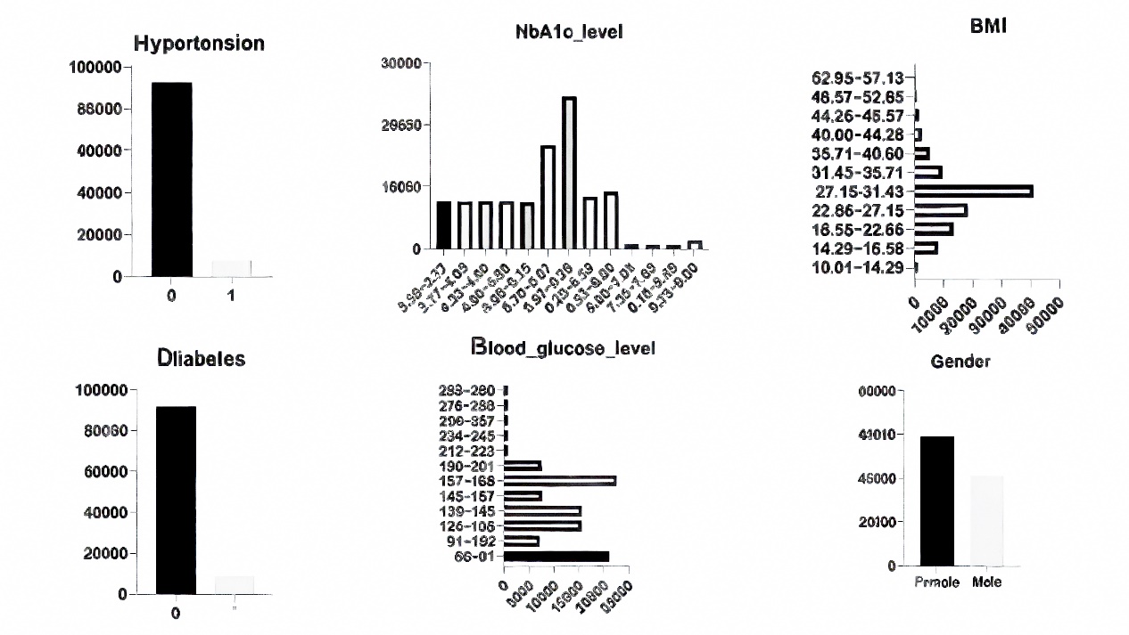
Figure 1. Data analysis and distribution

3.2. Data prepressing

3.2.1. Feature analysis and data visualization

Before data preprocessing, data mining and feature analysis are performed to understand the distribution of data, relationship between features, etc. through visualization and statistical methods. Correlation analysis of variable traits is a common data mining technique that visualizes the degree of correlation between traits by calculating correlation coefficients between traits and visualizing the correlation results in the form of heat maps. Such analyses provide a better understanding of the data and guide subsequent modeling and feature selection (Figure 2).

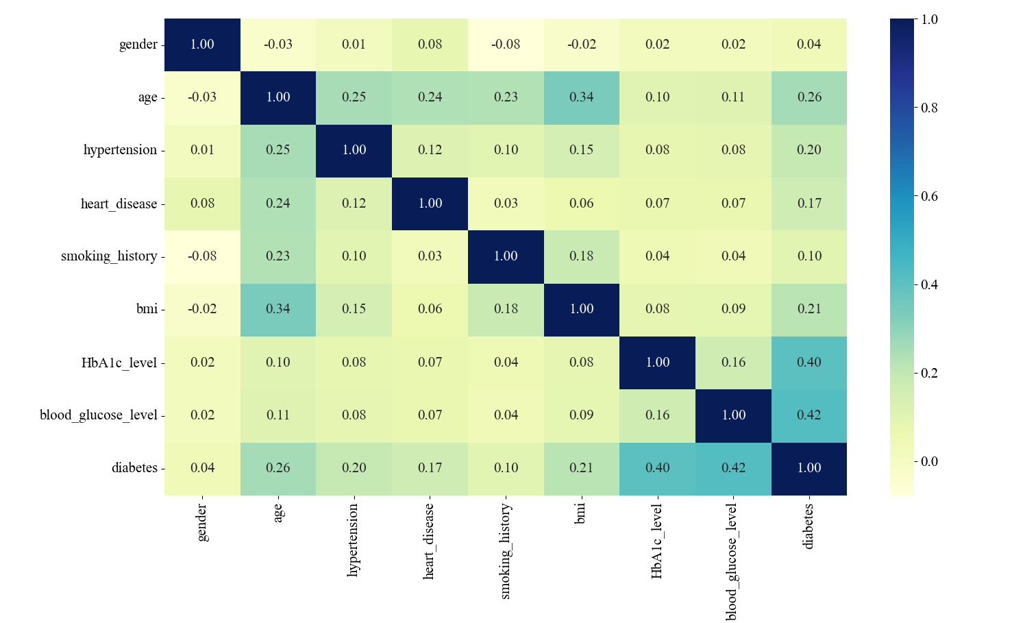
Figure 2. Correlation matrix of features

The variables blood glucose level and HbA1c_level were relatively highly correlated with diabetes, with 0.40 and 0.42, respectively. In the correlation analysis between the characteristic variables, the correlation between the two variables, bmi and age, is the highest, and there is a certain degree of linear relationship, but the correlation is not very strong, so in the experimental data processing, the effect of the correlation between the two can be ignored (Figure 3).

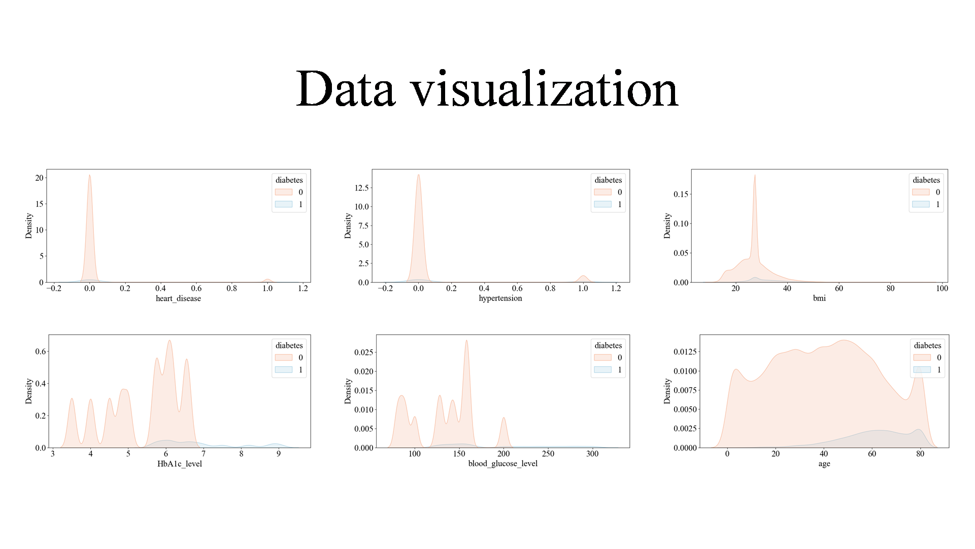
Figure 3. Data visualization

3.2.2. Data preprocessing

3.2.2.1. Data Cleaning

Handling Missing Values: Fill in missing values, either by replacing them with means, medians, plurals, etc., or by using interpolation methods. Handling outliers: Detect and handle outliers, which can be identified and handled through statistical or model-based methods, such as truncation, deletion, or replacement. Handling duplicate values: Remove duplicate samples or features to avoid adverse effects on model training.

There were no NA values in this dataset. For smoking_history variable there is category that defines if there is information about patients smoking history. We firstly got a view of categorical variables in this dataset (Figure 4).

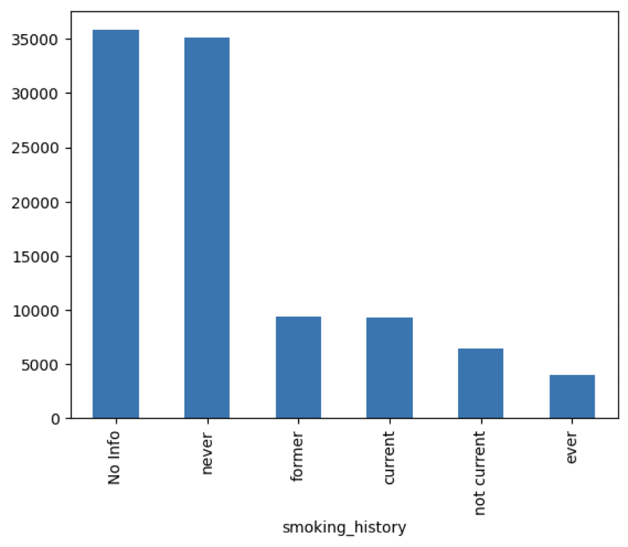
Figure 4. Smoking_History of cases in the dataset

There is a lot of people from whom we did not get the information about smoking habits. Because of that we leave that category in variable. We can consider grouping other categories that are not so frequent, but for now we leave this variable as it is. Also, we have checked their correlation between output and this variable with chi2 test and results are saying that there is significant correlation between those two.

There exists other category, supposedly an error in data gathering. Because the lack of correlation between gender and other variables, we cannot fix by these values by hand. Because there are only 18 other values, we will set them to most frequent category as Female.

We have also used chi2 test to find out if there is correlation between output and these variables, and there surely is. After finishing review of categorical data, we can proceed on analyzing numerical data. Because there is binary values and ordinary numerical values, we had two separate analyses (Figure 5).

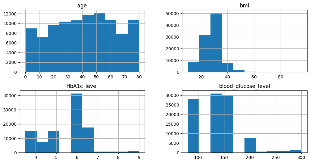
Figure 5. Data distribution of the dataset

Variable bmi has many outliers. We will leave them for now, because we must consider a multivariable outlier analysis later. Other variables have normal results, some of which have few outliers, but nothing strange. We can continue analyzing binary variables.

First, we have huge class imbalance in this dataset, where only 5% of the people have diabetes. So, the accuracy for this classification problem will not be useful for evaluation. Also, there is correlation between output and input binary variables with Pearson correlation coefficient. This is important because these variables have high impact on output. Next stage is transforming categorical into numerical data.

3.2.2.2. Data Transformation and splitting

Feature encoding: in this experiment, One-Hot Encoding was used for feature encoding to improve the performance and generalization of machine learning models. Dividing the dataset into training, validation, and testing sets, 70% of the data were used for training, 15% for validation tuning, and 15% for final model evaluation in this experiment.

Because gender was binary categorical variable we used binary conversion, where Female now have value 1, and Male now have value 0. For smoking_history variable we used OneHotEncoder and made 5 new columns, for each unique value of this variable. Last thing to do for preprocessing data was to normalize it. Because there is a lot of columns that is made from OneHotEncoder, for normalization we used MinMaxScaler. Our preprocessing was finished and we can now focus on anomaly detection. Before that we need to separate train, validation and test set for further modeling.

3.3. Models

3.3.1. XGBoost

XGBoost is a versatile and portable library designed for efficient distributed gradient-based decision boosting. Developed by Dr. Tianqi Chen from the University of Washington, XGBoost is built upon the gradient boosting decision tree (GBDT) algorithm. In GBDT, a tree is trained with the training set and the true values of the samples, and the predictions from this tree are subtracted from the true values to calculate residuals. Subsequently, a new tree is trained using these residuals as the new target variable instead of the original true values. This process is repeated iteratively, with each new tree learning to predict the residuals from the ensemble of previous trees. The number of trees in the model can be specified manually, and training can be monitored and stopped based on various metrics such as validation set error.

When predicting new samples, each tree in XGBoost is given an initial value that is combined to produce the final sample prediction, yielding superior performance compared to the conventional GBDT algorithm. Unlike the GBDT algorithm, which relies solely on first-order derivative information, XGBoost employs a second-order Taylor decomposition of the loss function, leading to a more efficient and less error-prone optimal solution. By incorporating a regular term in the function, XGBoost reduces the model's variance, resulting in a simpler trained model that mitigates overfitting issues.

3.3.2. Other models

In our study, we used 7 in models for data analysis comparison study, they were Logistic Regression (LR), Random Forest (RF), Decision Trees (DT), Gradient Boosting Decision Trees (GBDT), AdaBoost and Neural Networks (NN).

3.4. Experimental setup

We divided the data into a training set and a test set. We used 3000 cases in the training phase dataset to access train and validate the XGBoost models. We then used 27,000 patients in the test phase dataset to evaluate their performance.

The hyperparameters in the experiment, epochs were 50, batch_size was 100. When the Batch Size is adjusted to be larger, the number of iterations (updates) within an Epoch is reduced accordingly, and an underfitting state will occur. To prevent this, the number of Epochs should be increased. For every of the sets,we use the GridSearchCV method for hyperparameter optimization and a cross-validation strategy for model evaluation. Four grid search objects gridTree, gridKNN, gridLogistic, and gridBoost were created for parameter tuning of the decision tree classifier, K-nearest neighbor classifier, logistic regression model, and gradient boosting classifier, respectively. Each grid search object specifies a different parameter grid and cross-validation fold. Among them, in DT, for the three parameters, ‘min_samples_leaf,max_depth, min_samples_split’, three parameters were tuned, while the cross-validation fold was set to 3, the cross-validation fold of KNN was set to 5, while ‘n_estimators’ was specified; the cross-validation fold of Logistic was 5, while ‘param_grid’ was specified. Boost cross-validation fold of 3 with ‘learning _rate’ and ‘n_estimators’ specified.

3.5. Assessment metrics

The accuracy, precision, recall, AUC, F1 were used as assessment metrics in this study. In the following formulas, the first letter indicates the rightness or wrongness of the prediction whereT is correct and F is wrong. And the second letter indicates the category of the prediction where-P is the positive category and N is the negative category. Set the number of positive samples to be M and the number of negative samples to be N,also i belongs to the set of positive sample numbers.

\( Precise=P=\frac{TP}{Predicted Positive}=\frac{TP}{TP+FP}\ \ \ (1) \)

\( Recall=R=\frac{TP}{Actual Positive}=\frac{TP}{TP+FN}\ \ \ (2) \)

\( F1=\frac{2}{\frac{1}{R}+\frac{1}{P}}=\frac{2*P*R}{P+R}=\frac{2TP}{2TP+FP+FN}\ \ \ (3) \)

\( Accuracy=A==\frac{TP+TN}{TP+FP+FR+TN}\ \ \ (4) \)

\( AUC=\frac{\sum ran{k_{i}}-\frac{M(1+M)}{2}}{M*N}\ \ \ (5) \)

To find combinations where positive sample scores surpass negative ones, assuming all positive scores are higher, we assigned rank n to the highest score combination. However, among n-1 lower ranks, M-1 combinations of positive samples aren’t tallied (for simplicity). Subtracting these gives M * (M +1)/2. This formula holds when positive scores exceed negatives, yielding AUC 1.

Rank value represents combinations with minimal score differences. Subtracting (positive, positive) groups yields the formula. Equal scores receive equal ranks, averaging ranks of same-score samples regardless of class distinction.

4. Results and discussion

4.1. Results

In this study, a diabetes dataset with 8 feature variables and 30,000 samples was selected for diabetes diagnosis research. An XGBoost-based data training model was developed by training and prediction with deep neural networks, visualization of network training. The final model achieved accuracy (97%), precision (93%), and recall (99%). This study realized the diagnosis of diabetes mellitus by deep neural network, and achieved certain research results, which is more convenient for the diagnosis of diabetes mellitus, and can over effectively reduce the medical cost and improve the diagnostic efficiency.

XGBoost’s accuracy is 0.97, recall0 is 0.99, precision is 0.93, f11 is 0.8, and f10 is 0.98, which, taken together, shows that XGBoost’s correctness is relatively high, and some of the precision rates and accuracy substantially outperforms the other models. According to our study results XGBoost’s prediction correctness is relatively good, proving that compared to other models XGBoost has the most excellent prediction correctness for unsupervised learning with multiple data (Table 2).

Table 2. The results of models

4.2. Discussion

In the various model metrics of this experiment, XGBoost has better performance compared to GBDT and other models, such as accuracy, recall, F11, and especially precision. The accuracy, AUC, precision1, recall1, and F11 are 0.97, 0.98, 0.94, 0.7 and 0.8, respectively. Comparison between Gradient Boosting Decision Trees (GBDT) and XGBoost (XGB) can be based on factors such as sampling techniques, tree depth, base learner, implementation of serial and parallel processing, handling of missing values and anomalies, regularization methods, computational efficiency, result calculation approach, and accuracy metrics [18-19]. XGB shares similarities with Random Forests (RF) by incorporating column sampling to reduce computation time and overfitting, while GBDT uses all features. XGBoost can use CART regression tree or a linear classifier as its base learner, unlike GBDT limited to CART regression tree. XGBoost parallelizes feature selection, speeding up optimal split point search through pre-sorted features. It applies L1 and L2 regularization to leaf nodes, mitigating overfitting, and uses second-order Taylor expansion for more accurate loss curve fitting compared to GBDT's first-order gradient. XGBoost introduces Shrinkage to scale leaf node weights, aiding learning in subsequent stages. Practitioners often choose lower eta and higher iterations for better learning.

LR is suitable for discrete features, and the discretized features are robust to abnormal data. Logistic regression belongs to the generalized linear model, and the expression ability is limited; after the single variable is discretized into N, each variable has a separate weight, which is equivalent to the introduction of nonlinearity for the model, and can improve the model expression ability and increase the fitting. After discretization, feature crossover can be carried out, changing from M+N variables to M*N variables, further introducing nonlinearity and improving the expression ability. RF improves upon the decision tree algorithm by creating a forest of classification trees. It repeatedly selects k samples from the original training set N with replacement to form new training sets, then generates k trees based on these sets. Each tree contributes to the classification decision, and the final result is determined by a voting mechanism. This approach reduces overfitting as each tree is trained on a different subset of data. Notably, random forest uses two random sampling processes: row sampling (with replacement) and column sampling (m features selected from M). This randomness prevents overfitting, eliminating the need for pruning. Each decision tree is built until leaf nodes are pure or cannot split further. The combination of many diverse trees allows for robust classification, enhancing accuracy and reducing bias.

Decision trees segment samples by hierarchical progression of attribute judgments. Decision trees can do the job of fitting to the training set, but an overfitted model has no value for the test samples, so branches need to be cut to reduce the risk of overfitting. By setting up a validation set for the model, the decision tree's performance on the validation set determines which branches to cut. GBDT has more nonlinear transformations, strong expressive ability, and does not need to do complex feature engineering and feature transformation. The disadvantages of GBDT are also evident, The Boost algorithm executes sequentially, which is not conducive to parallelization, resulting in high computational complexity. Additionally, it is not well-suited for processing high-dimensional sparse features. Traditional GBDT only uses the first order derivative information in optimization. AdaBoost's adaptiveness is demonstrated by reweighting the misclassified samples from the previous basic classifier and using them to train the subsequent one. Additionally, a new weak classifier is introduced in each iteration until a sufficiently low error rate is achieved or a predefined maximum number of iterations is reached. In the present study, the training process of an NN is an iterative one, where the initialization can be thought of as randomly obtaining individual weights and then each iteration. The input samples enter each neuron of the current NN, weighted with the existing weights, and then output by the activation function to the neurons connected later. This progresses layer by layer, culminating in the output of the overall network of the NN. The output of this run is compared to the target, the Cost is calculated, and then the weights of each layer and neuron of the network are back-adjusted by minimizing the Cost. This iteration is repeated until convergence.

The dataset is small with only 8 feature variables, limiting neural networks' effectiveness due to potential overfitting and the inability to leverage high-dimensional cross-features. Model structure and training parameter selection are time-consuming for such data. Conversely, tree models are suitable for small datasets, focusing on manually identifying key features. Boosting algorithms work well for tabular data, while deep learning is better for large non-tabular datasets [20]. Deep learning’s strength lies in automatically generating hidden features for complex data, although it’s less efficient than gradient boosting trees. Deep learning surpasses gradient boosting for tabular data but requires significant time for network tuning. When tabular data lacks a clear pattern, neural networks may need inefficient fully connected networks, making traditional machine learning models and task-tailored networks like DeepFM more practical [21].

There are some limitations in the present study that need to be urgently addressed in future research to improve the performance of the models and the accuracy of the predictions. First, the problem of insufficient data sample size, which is the main limiting factor of current machine learning models, should be addressed. The dataset used in this experiment is 30,000 pieces of data with 8 feature variables, which is a small amount of data that has an impact on the accuracy of the experiment. Second, considering the limited data sources and the need to consider the issue of patient privacy, the current publicly available datasets in the market are not continuously updated and have a small amount of data, other datasets should be explored for inclusion in our analysis to expand our data resources. For example, adding information related to whether there is a family history of diabetes or lifestyle habits is also an option.

5. Conclusion

Diabetes has always been a closely watched disease, and this study is of great significance for the prediction of diabetes based on XGBoost. Under the conditons of the dataset used in this experiment, data preprocessing and visualization are performed first, using the GridSearchCV approach to optimize the hyperparameters for each collection and then by comparing the performance of XGBoost with the other six models, in which XGBoost has a better result compared to the other models. The final model achieved accuracy of 97%, precision of 93%, and recall of 99%.In summary, this study is based on XGBoost to predict diabetes mellitus, which is clinically useful for doctors to diagnose patients.

Authors Contribution

All the authors contributed equally and their names were listed in alphabetical order.

References

[1]. Lovic DP, Alexia Z, Ioanna G, Haralambos P, Andreas M and Athanasios 2020 The Growing Epidemic of Diabetes Mellitus Current Vascular Pharmacology 18 2
[2]. Segar M W, Vaduganathan M, Patel K V ,et al. 2019 Machine Learning to Predict the Risk of Incident Heart Failure Hospitalization Among Patients With Diabetes: The WATCH-DM Risk Score Diabetes Care 42 2298-2306
[3]. Ostrander J R, Leon D, Thomas F J R, Norman S H, Marcus O K and Frederick H E 1965 The relationship of cardiovascular disease to hyperglycemia Annals Internal medicine 62 1188-98
[4]. Badiger, Sharan, Prema T A and Utkarsha N 2013 Hyperglycemia and stroke International Journal of Stroke Research 1 1-6
[5]. Vincent, Andrea M, Lisa L M, Carey B and Eva L 2005 Short‐term hyperglycemia produces oxidative damage and apoptosis in neurons The FASEB Journal 19 1-24
[6]. Emerging Risk Factors Collaboration, Sarwar N, Gao P, et al. 2010 Diabetes mellitus, fasting blood glucose concentration, and risk of vascular disease Lancet 375 2215-22
[7]. Kavakiotis, Ioannis, Olga T, Athanasios S, Nicos M, Ioannis V and Ioanna C 2017 Machine Learning and Data Mining Methods in Diabetes Research Computational and Structural Biotechnology Journal 104–16
[8]. Li M, Fu X and Li D 2020 Diabetes prediction based on XGBoost algorithm In IOP conference series: materials science and engineering 768 072093
[9]. M A R Refat, M A Amin, C Kaushal, M N Yeasmin and M. K 2021 International Conference on Signal Processing Islam 6th International Conference on Signal Processing, Computing and Control 654-9
[10]. D. Çalisir,andE. Dogantekin 2011 Differential sequential patterns supporting insulin therapy of new-onset type 1 diabetes Expert Systems with Applications 38 8311-5
[11]. Kevin Plis, Razvan Bunescu and Cindy Marling 2014 A Machine Learning Approach to Predicting Blood Glucose Levels for Diabetes Management Modern Artificial Intelligence for Health Analytics AAAI-14
[12]. Juyoung Lee, Bhumsuk Keam, Eun Jung Jang, Mi Sun Park, Ji Young Lee, Dan Bi Kim, Chang-Hoon Lee, Tak Kim, Bermseok Oh, Heon Jin Park, Kyu-Bum Kwack, Chaeshin Chu and -Lae Kim 2011 Development of a Predictive Model for Type 2 Diabetes Mellitus Using Genetic and Clinical Data 2 Public Health Res Perspect 2011 75-82
[13]. Rafał Deja, Wojciech Froelich and Grazyna Deja 2015 Differential sequential patterns supporting insulin therapy of new-onset type 1 diabetes BioMedical Engineering OnLine 14 13
[14]. Aileen P. Wright, Adam T. Wright, Allison. McCoy and Sittig 2015 The use of sequential pattern mining to predict next prescribed medications Journal of Biomedical Informatics 53 73–80
[15]. V. Lagani, F. Chiarugi, S. Thomson, J. Fursse, E. Lakasing, R.W. Jones, et al. 2015 Development and validation of risk assessment models for diabetes-related complications based on the DCCT/EDIC data J Diabetes Complications, 29 (4) (May-Jun 2015), pp. 479-487
[16]. V. Lagani, F. Chiarugi, D. Manousos, V. Verma, J. Fursse, K. Marias, et al. 2015 Realization of a service for the long-term risk assessment of diabetes-related complications J Diabetes Complications, 29 (5) (Jul 2015), pp. 691-698
[17]. L. Sacchi, A. Dagliati, D. Segagni, P. Leporati, L. Chiovato, and R. Bellazzi 2015 Improving risk-stratification of diabetes complications using temporal data mining Conf Proc IEEE Eng Med Biol Soc, 2015 (Aug 2015), pp. 2131-2134
[18]. Chen T and Guestrin C 2016 XGBoost: A Scalable Tree Boosting System ACM
[19]. Liang W, Sui L, Guo Z and Hao W 2020 Predicting Hard Rock Pillar Stability Using GBDT, XGBoost, and LightGBM Algorithms Mathematics 8 765
[20]. J Wu, Y Li and Y. Ma 2021 Comparison of XGBoost and the Neural Network model on the class-balanced datasets IEEE 3rd International Conference on Frontiers Technology of Information and Computer 457-61
[21]. Giannakas F, Troussas C, Krouska A, Sgouropoulou C and Voyiatzis I 2021 XGBoost and Deep Neural Network Comparison: The Case of Teams’ Performance (Cham: Springer)
Cite this article
Xie,P.;Xu,J. (2024). Prediction of diabetes mellitus using XGBoost model. Applied and Computational Engineering,67,131-141.
Data availability
The datasets used and/or analyzed during the current study will be available from the authors upon reasonable request.
Disclaimer/Publisher's Note
The statements, opinions and data contained in all publications are solely those of the individual author(s) and contributor(s) and not of EWA Publishing and/or the editor(s). EWA Publishing and/or the editor(s) disclaim responsibility for any injury to people or property resulting from any ideas, methods, instructions or products referred to in the content.
About volume
Volume title: Proceedings of the 2nd International Conference on Software Engineering and Machine Learning
© 2024 by the author(s). Licensee EWA Publishing, Oxford, UK. This article is an open access article distributed under the terms and
conditions of the Creative Commons Attribution (CC BY) license. Authors who
publish this series agree to the following terms:
1. Authors retain copyright and grant the series right of first publication with the work simultaneously licensed under a Creative Commons
Attribution License that allows others to share the work with an acknowledgment of the work's authorship and initial publication in this
series.
2. Authors are able to enter into separate, additional contractual arrangements for the non-exclusive distribution of the series's published
version of the work (e.g., post it to an institutional repository or publish it in a book), with an acknowledgment of its initial
publication in this series.
3. Authors are permitted and encouraged to post their work online (e.g., in institutional repositories or on their website) prior to and
during the submission process, as it can lead to productive exchanges, as well as earlier and greater citation of published work (See
Open access policy for details).