1. Introduction

In the realm of game development, a fascinating interplay between algorithms and creativity converges to create immersive digital experiences that captivate players' minds and challenge their skills. Commonly, Mazes and labyrinths take up a significant part in electronic games. It engages players by encouraging deeper exploration into the expansive world of the game. We fully acknowledge this importance, which inspires us to use mazes as the foundation and the priority of our work to show how a 2D game are built.

There exists many complete and detailed works that explain some of the algorithms involved in games, such as “Analysis of maze generating algorithms” by Peter Gabrovšek. [1] In the essay, the author introduces and compares a number of maze generating algorithms. However, pure analysis on the algorithms themselves may cause a lack of understanding among the beginners who want to learn the implementation of algorithms in games. Our work links the algorithms with actual code as well as compares the performance of several mainstream maze generation algorithms in our independent game quantitatively, which makes the illustration clearer.

In the code part, we focus on the utilization of Pygame -- a Python module tailored for crafting 2D games. Pygame is a prominent player in the landscape of game development, which offers a versatile platform for aspiring game designers. Built upon the Python programming language, Pygame boasts an accessible and cost-free framework, making it an ideal choice for those new to game creation.

This essay embarks on a journey into the intricate world of game design, where the spotlight is cast on the cardinal algorithms implemented in a small yet captivating Pygame-based game. The ideal function of the game is to move a character through a maze while gaining points. Our focus lies squarely on the ingenious algorithms that breathe life into this digital realm. As the digital tapestry of the game unfolds, this essay explores the profound impact of algorithmic intricacies on the player's engagement and the potential for these concepts to transcend the confines of simplicity. By using the context of a 2D game, we will be able to explain the mechanisms through which various algorithms interact to form a complete electronic game.

2. Maze Generation

In this essay, a maze is considered as a giant rectangle consisting of small squares. These squares are called cells. Each cell has its neighbors: north, south, east and west. At the start, all the cells are not connected to each other, which means there is a wall between each cell and its neighbors Consider a maze with m rows and n columns, then the number of cells should be m*n. For instance, if a maze consists of 24 rows and 32 columns, then the default maze without any adjustments should look similar to figure 1. With the original maze, we can now apply maze generating algorithms to remove walls(or carve paths) between cells to create the labyrinth. In this part we are going to introduce various maze generation algorithms and compare them to find out which is the most suitable for the game. In addition, we will look at the code realizations in Python.

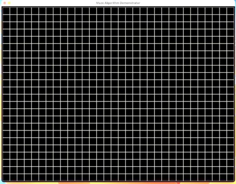
Figure 1. Default Maze

2.1. Binary Tree

The first thing to admit is that Binary Tree is a basic algorithm, so that we start our discussion with that. In a Binary Tree program, we iterate through all the cells in the grid, each time randomly choosing between the north and east neighbors and connect to them. If a cell does not have a north neighbor, then connect it to its east neighbor, and vice versa. If the cell have neither a north neighbor not an east neighbor, then we leave it alone.

Now we understand the logics, we should turn to the code implementation. We used a Cell class and a Grid class to store the related data. The Cell class describes a single cell, allowing a cell object to link to its neighbors. It contains a link method and a neighbors method that returns the neighbors of the cell. A cell object has attributes that describes the position of the cell. The Grid class describes a grid containing the cells, the cell objects are stored in a 2D-array. These classes will also be used for the introduction of other maze algorithms. In addition, we wrote a markup class to keep track of other information in each cell such as whether it’s visited.

Now we can use the two classes to write the Binary Tree function. The grid object is passed as a parameter to the function so we could modify it. We use a for loop to iterate through the cells, implement some if-statements to cope with different situations, and then randomly choose to connect the cells.

The result of the algorithm is as shown in Figure 2. It’s worth noting that the code for showing maze is not displayed yet, but we will be discussing it later in the work. As Figure 2 shows, the program generates a perfect maze, with each cell linking to either its north or east neighbors. Binary Tree is probably the easiest algorithm to generate mazes in terms of logic and code. Each cell can be handled in parallel. However, due to its simplicity, the maze constructed are usually biased for diagonal flow. This means that if we put a character in the maze, it will be easier for it to move diagonally from the south west corner to the north east corner and vice versa. For the game, we do not want the movement of the player to be confined in one direction, therefore we will not apply this algorithm.

Despite its flaws, the Binary Tree provides beginners with a basic understanding of how maze algorithms work. This will be helpful for learning the following, more complex algorithms.

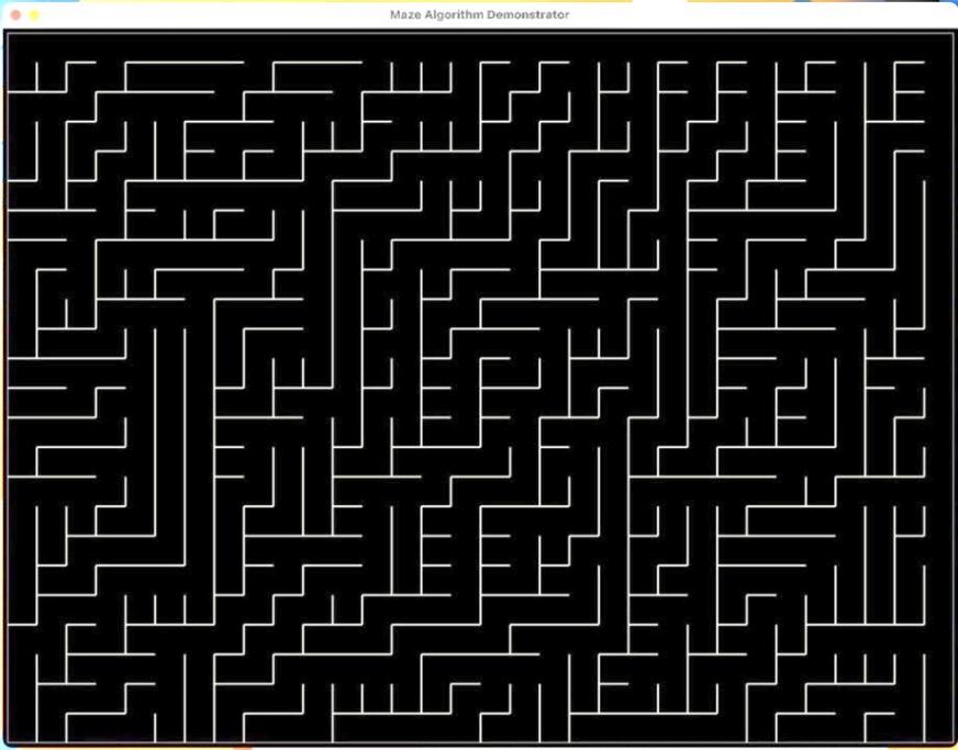
Figure 2. Maze generated using Binary Tree

2.2. Aldous Broder Random Walk & Wilson’s Random Walk

Aldous Broder starts from a random cell(v), marks it as visited, and repeats the following steps [1]:

Choose a random neighbour u of v (not necessarily unvisited).

If u is not visited visit it, and connect it with v.

1. Set v as u.

The process ends when every cell in the grid has been visited.

With that, we could be able to implement it in the code. We used the Markup class to keep track of the cells in terms of whether they have been visited. We used an infinite while loop to repeat the procedures and adds an if statement to break the loop when all the cells are marked visited.

Wilson’s algorithm is similar to Aldous Broder in many ways. It starts with a random cell, marks it as visited, and repeats the following steps:

1. Choose a random unvisited cell as a starting point

2. Perform a loop-erased random walk, choosing a random neighbor at each step

3. If the random neighbor has been visited, the walk is over. Now mark all the cells from the walk as visited, and link all of them in the order they were chosen.

The process ends when every cell in the grid has been visited.

Loop-erased walk: A loop occurs when the next cell chosen is the same cell as one in the path of this walk. Loop-erased random walk on the integer lattice is, a process obtained from simple random walk by erasing the loops chronologically. The process has self-avoiding paths [2]. This means when the program encounters with a loop, it erases the loop from the path, retaining the beginning of the loop.

In our code, the loop-erasing function is achieved by using a path list to store the visited cells in one walk and examine whether the next cell picked is in the path. If so, then we use the slicing method to erase the loop and start from the beginning of this loop.

The results(Figures 3-4) of the two algorithms have similar appearances. They both generates perfect mazes that are unbiased. It’s impossible to tell from the output if the maze is generated by Aldous Broder or Wilson’s. Although the graph seems suitable for the game, its performance is sometimes considered inefficient.

For Aldous Broder, the program starts quick, walking through the grid randomly. However, it does not finish the job neatly, since it is possible to take a long time to randomly walk to the last few cells that are not visited. If we put an iteration count in the function and print the number of steps accomplished, we could see that for a maze containing 768 cells, Aldous Broder took 12536 steps to complete it (Table 1). The workload is relatively large for a maze this size.

On the other hand, for Wilson’s, the program has a rather slow beginning, since loops occur easily when randomly walking through an empty grid. Fortunately, the advantage of this algorithm is that it does a quick job in the end, choosing the unvisited cells at an instant without the possibility of traveling through visited cells like in Aldous Broder. Still, the calculations needed is a giant value. As shown in Table 1, 3346 random cells were chosen and 943 loops were removed.

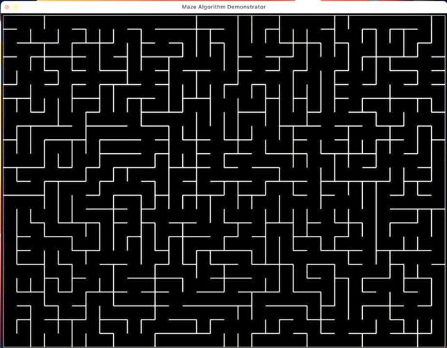
Figure 3. Maze generated using Aldous Broder

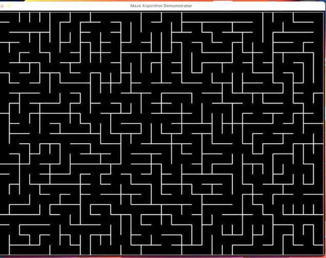
Figure 4. Maze generated using Wilson’s

Table 1. Properties table of Maze algorithm

2.3. Recursive Backtracker

As the name implies, it uses recursion, but the code does not necessarily need to embody recursion. Algorithm starts recursive function for every neighboring position that can be moved to. If it has no unvisited place to move to it has to go back the way it came until it reaches position that allows it to move in a direction it has never been through [3]. Whenever there appears a neighbor that is unvisited while you back up along the path, you link to and move to that cell. This algorithm requires some additional state -- you need to keep track of the cells you have visited, in reverse order. Therefore, we need a stack(a last-in, first-out data structure). We used an explicit stack, where a list is used as a stack. Instead of calling a function multiple times, we used loops and a Boolean value “flag” to keep track of the status of the current cell’s neighbors. The result is in Figure 5. This algorithm leads to mazes with long, twisty paths with few dead ends. However, Recursive Backtracker has its own drawbacks. The algorithm is not very memory efficient. It has to keep a stack, which may contain every cell in the entire maze. In addition, most programming environments have limits on recursion depth to avoid stack overflow. This limits usage of recursion in bigger labyrinth or forces programming in such a way to take this limit into consideration [3].

2.4. Decision

For this particular game, we need to set special trophies at a cell where the player cannot easily get to. In other words, we need the longest path in the maze to be long and twisty. This is the reason that we choose to use Recursive Backtracker, since it produces mazes with longer paths (Table 1).

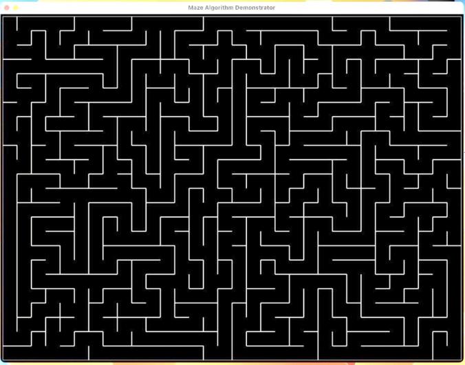
Figure 5. Maze generated using Recursive Backtracker

2.5. Visualization

Now we have the suitable algorithm for mazes, we will focus on the visualization of the maze. In Pygame, images are drawn or printed on surfaces. We initialize the display surface to a size of 1034*778 pixels(Figure 1). Under this measurement, for a 24 * 32 grid, the side length of a cell is 32. Therefore we get the function for the x and y coordinates of the start of a cell:

\( cel{l_{x}}=col*32+5 (1) \)

\( cel{l_{y}}=row*32+5 (2) \)

where col is the column number of the cell and row is the row number of the cell. Using these coordinates and the data stored in the Cell and Grid class, we could draw the walls between cells using the Python module gfxdraw. Displaying the surface with different algorithms implemented in the game loop would lead to the various results as shown above in Figures 2, 3 and 4.

The maze part of the game is mostly accomplished at this point. Now it’s time to turn to the characters and control part of the game.

3. Printing Characters

The characters and items in the game are made by the sprite module in pygame, which manages and stores them well [4]. In the design idea of our game, sprites can be classified into two types which are static sprites and dynamic sprites. Static sprites included: Tricky Ghost (slows down the opponent's movement speed), Eternal Heart (cancels out a spell on you and bounces the effect), and so on. These ordinary prints are relatively simple, just make a pixel item and print it with the blit() statement. The dynamic sprite part is a lot more complicated. Firstly, We need to get an image of the pixel character that included every frame. We mainly draw it with PS, as shown in Figure 6.

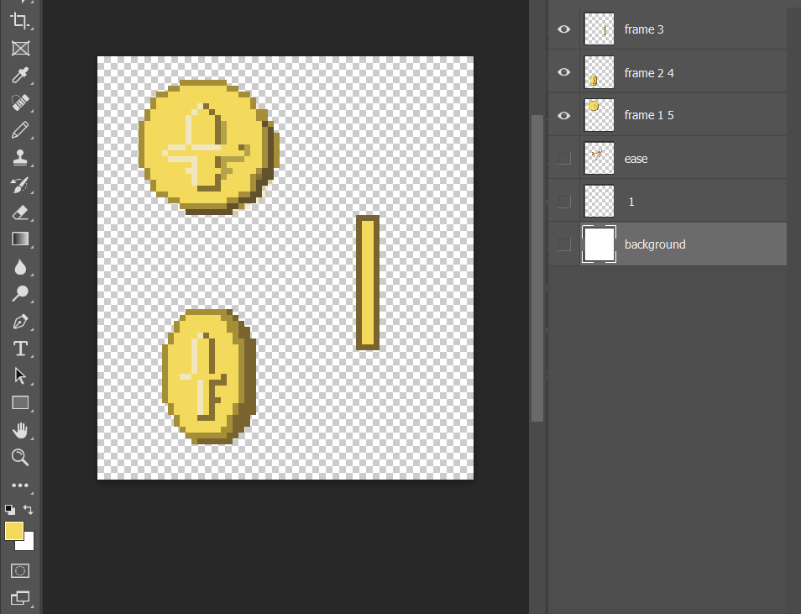
Figure 6. The process of drawing gold coins with PS

Secondly, We use software PS to help me find the coordinates of the upper left vertex corresponding to each frame of the character and the length and width of the rectangle. After everything is in place, We use arrays to store information for each frame and initialize a variable “current_image_index” to achieve loop control of the array of frames from 0 to the number of frames by adding one to each loop and taking the remainder of the total number of frames. Then adjust the range of images you want to print through the area parameter in blit(souce, dest, area=None, special_flages=0). From this, the character's standby action is made. It is worth mentioning that not all image materials have transparent backgrounds, pygame.Surface.set_colorkey() is a good way to set the background of the footage to transparent. Figure 7 shows the effect what the printing code performanced in the maze game.

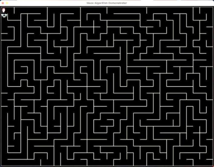
Figure 7. Characters print in maze game

4. Character Movement

First, pygame and random modules are imported at the beginning of the code. As the rules of the game designed, initial positions of 2 characters are selected randomly in the maze where random module is used. Random.randinit() function is invoked to choose a starting position within the size of the maze.

The initial setting of running is True, and clock = pygame.time. Clock is used to control the rate of frame change in the loop. In this light, players are able to run their games consistently across different devices although they may be with quite different processing speed. The above mentioned code goes with clock.tick(60), which means the frame rate is limited specifically at 10 Frames per second (FPS).

In the main game loop, the line ‘for event in pygame.event.get()’ demands to iterate all events that are in the event queue currently, which holds all events created by players, allowing the program to respond to players appropriately.

Valid movement is defined in order to monitor the scope of characters’ movements, avoiding moving out of the maze.

In order to get the keyboard control, we set ‘keys=pygame.key.get_pressed()’. All states of the keyboard are checked when this line is called. In this way, players are able to control characters on their keyboards.

Specifically, player 1 controls character 1 which is represented as char1 in the code using up, down, left and right keys to control the character movement during the game. Similarly, player 2 controls character 2 which is represented as char2 in the code using W, S, A, and D [5].

As the rule is designed, each pressing each key once conducts one movement of a character each time. The goal of players is to gain coins as many as possible to beat their component by controlling characters’ movements.

At the end of the game loop, the line ‘pygame.display.flip()’ is used to update the game status and therefore update the positions of the characters.

5. Using Longest Path to Place Trophies

5.1. Find the Longest Path

We use the longest path in the maze to help us place important trophies for the players to earn points.

In order to find the longest path in any mazes, Dijkstra’s algorithm is used twice. Dijkstra's algorithm (named after its discover, E.W. Dijkstra) solves the problem of finding the shortest path from a point in a graph (the source) to a destination [6].

The procedures for Dijkstra is as follows:

1. Mark the root cell with zero

2. Create a frontier to hold cells and put the root cell in it

3. Repeat until the frontier is empty:

(1) Find the cell with the smallest value, we call it c

(2) Remove c from the frontier

(3) Find all neighbors connected to c and mark them with 1+c’s value. Add them to the frontier

Dijkstra marks every cell with a cost value that is useful to find the longest path [7].

This is the outline of the longest path algorithm.

(1) Pick a random cell for the root from the maze, which can be called cell A.

(2) Run Dijkstra’s algorithm on A.

(3) Since we know the cell that has the highest markup is the farthest cell from cell A, which can be called cell B.

(4) Run Dijkstra’s algorithm on cell B to run the highest markup on this second run, which can be called cell C

(5) Generally, the longest path in the maze is from cell B to cell C

(6) As the game is designed, reward can be put in the farthest cell to make the game more challenging and complex.

5.2. Effect of Trophies

The icon of the trophy is placed at one of the ends of the longest path, where 2 characters start at the other end of the longest path. The special effect of the trophy is designed that if character 1 reaches the trophy first, the speed of character 2 will be slower. Therefore, character 2 may collect less coins than character 1. The rule is valid because both players want to get this trophy first, or they might lose.

5.3. Evaluation

Longest path can be used to evaluate the complexity of a maze, which means the longer the longest path, the more complex the maze [8].

Specifically, the Dijkstra function initializes the distance from the origin to origin as 0 and creates a queue in the form [(distance, cell)] to save data. Distance here in the code represents markup. Also, ‘distance’ is a dictionary that stores values that indicates the distances from the cell to the origin. As the Dijkstra algorithm is running, if the current markup of the cell is greater than the value store in the markups dictionary, we use ‘continue’ demand to skip processing the cell again. If a shorter distance is found, the distance dictionary is updated.

6. Collision Check Between Characters and Coins

As the rules of the game are designed, coins are scattered randomly in the maze. Movements of characters are controlled by keyboard. When characters move to the same coordinate as the coins, the coin will disappear and this player get 1 point.

Initially, the score of both players is set as 0. By comparing the final scores of them, the winner is determined as the one with a higher score. For detecting the collision, ‘for loop’ is used in the code to check the x-coordinate and y-coordinate of character 1 and character 2 with the coins respectively [9]. If both of them are equal, ‘coins.remove(coin)’ is used to remove the single coin from the ‘coins’ group, and then the for loop is set break [10].

7. Conclusion

In conclusion, this essay provided a comprehensive exploration of the interplay between algorithms and creativity in maze-based game design. The emphasis of this work is mainly directed on the realization of various algorithms, and serves as a testament to the dynamic and multifaceted nature of game development. Different from most of the previous works, this essay illustrates the usually incomprehensible concepts using an example of a real game, thus making the paper an interesting and comprehensive work for beginners or researchers. This work examined the maze-generating and solving algorithms, collision detection, as well as materializing character movement using Python. Details involving the game rules and specific effects are also noted. By bridging theoretical concepts with practical implementations and showcasing the utilization of Pygame, it illustrated how algorithms breathe life into digital experiences. We hold a hopeful attitude toward the future of electronic games and the algorithms involved, and believe that more efficient and straightforward algorithms or tools will be invented in the near future. In essence, while this essay gives a brief understanding of how algorithms and creative design come together to make engaging electronic games, it also provides an essential basis for later researches and experiments in the field of game developing.

Acknowledgement

Jiachen Piao, Xinyuan Hu and Qixuan Zhou contributed equally to this work and should be considered co-first authors.

References

[1]. Gabrovšek, Peter. "Analysis of maze generating algorithms." IPSI Transactions on Internet Research 15.1 (2019): 23-30.
[2]. Lawler, Gregory F. "Loop-erased random walk." Perplexing Problems in Probability: Festschrift in Honor of Harry Kesten(1999): 197-217.
[3]. Niemczyk, R., and Stanisław Zawiślak. "Review of Maze Solving Algorithms for 2D Maze and Their Visualisation." International Conference of Students, PhD Students and Young Scientists" Engineer of the XXI Century". Cham: Springer International Publishing, 2018.
[4]. DEV1 documentation. (2021). Pygame.sprite - pygame v2.0.1. https://www.pygame.org/docs/ref/sprite.html#pygame.sprite.Sprite.groups.
[5]. Lankoski P. “Player character engagement in computer games[J].” Games and Culture, 2011, 6(4): 291-311.
[6]. Javaid, Adeel. "Understanding Dijkstra's algorithm." Available at SSRN 2340905 (2013).
[7]. Widodo, Aris Puji (2007). “Simulasi Lintasan Terpendek Algoritma Dijkstea Berbasis Extensible Markup Language(XML)” http://eprints.undip.ac.id/1836/
[8]. Ryuhei Uehara & Yuchi Uno. “Efficient Algorithms for the Longest Path Problem.” In:fleischer, R., Trippen, G.(eds) Algorithms and Computation. ISAAC 2004. “Lecture Notes in Computer Science.”, vol 3341. Springer, Berlin, Heidelberg. https://doinorg/10.1007.978-3-540-30551-4_74
[9]. Teschner M, Heidelberger B, Müller M, et al. “Optimized spatial hashing for collision detection of deformable objects”[C]//Vmv. 2003, 3: 47-54.
[10]. van der Spuy R, van der Spuy R. “Making Sprites and a Scene Graph[J].” Advanced Game Design with HTML5 and JavaScript, 2015: 111-163.
Cite this article
Piao,J.;Hu,X.;Zhou,Q. (2024). Maze and navigation algorithms in game development. Applied and Computational Engineering,79,11-19.
Data availability
The datasets used and/or analyzed during the current study will be available from the authors upon reasonable request.
Disclaimer/Publisher's Note
The statements, opinions and data contained in all publications are solely those of the individual author(s) and contributor(s) and not of EWA Publishing and/or the editor(s). EWA Publishing and/or the editor(s) disclaim responsibility for any injury to people or property resulting from any ideas, methods, instructions or products referred to in the content.
About volume
Volume title: Proceedings of the 4th International Conference on Signal Processing and Machine Learning
© 2024 by the author(s). Licensee EWA Publishing, Oxford, UK. This article is an open access article distributed under the terms and
conditions of the Creative Commons Attribution (CC BY) license. Authors who
publish this series agree to the following terms:
1. Authors retain copyright and grant the series right of first publication with the work simultaneously licensed under a Creative Commons
Attribution License that allows others to share the work with an acknowledgment of the work's authorship and initial publication in this
series.
2. Authors are able to enter into separate, additional contractual arrangements for the non-exclusive distribution of the series's published
version of the work (e.g., post it to an institutional repository or publish it in a book), with an acknowledgment of its initial
publication in this series.
3. Authors are permitted and encouraged to post their work online (e.g., in institutional repositories or on their website) prior to and
during the submission process, as it can lead to productive exchanges, as well as earlier and greater citation of published work (See
Open access policy for details).