1. Introduction

In the digital age, as businesses strive to understand and cater to the evolving needs and preferences of their customers, the analysis of customers’ behaviors has emerged as a pivotal field of research. In the past years, behaviors built on people's trust, conversation, and trade records. However, with the development of technology, clickstream data has become the primary source for companies to study online customers’ preferences. It comprises the sequence of online actions taken by users as they navigate websites and digital platforms and represents a treasure trove of valuable information about user behavior, interaction, and engagement. Especially after the COVID-19, pandemic has turned people to prefer online shopping, which increased the need for new research to help businesses to predict customer behaviors based on clickstream data [1]. Also, when businesses predict the user’s shopping intents explicitly, they would offer customers more individual and fitted pages for users, which provide a satisfied and effective shopping experience for users [2]. Our research endeavors to explore customer behavior based on clickstream data and compare both machine learning and deep learning models' performance. By understanding how users navigate the digital landscape, businesses can decipher the intricate web of consumer preferences, effectively tailor their offerings, and, ultimately, foster lasting customer relationships.

Both machine learning and deep learning provide powerful tools for researchers to explore more conventions from customers and even preferences that are unrealized by users themselves. Machine learning, with its ability to discern hidden insights from vast datasets, offers the analytical prowess needed to extract meaningful information from the ever-expanding pool of clickstream data. And this definitely enforces the development of predictive models by adopting marketing research [1]. In past studies, researchers have applied machine learning to create personalized user experiences, detect unusual or fraudulent behavior, and evaluate the performance of different recommendation algorithms. As for deep learning, with its neural network architecture, it excels in capturing intricate relationships and extracting hierarchies of features that traditional machine learning approaches may struggle to reveal. Research indicates that deep learning has been used to predict the lifetime value of customers based on their past behavior, predict the likelihood of a user clicking on a particular ad, and create sophisticated customer journey maps by analyzing the sequence and context of customer interactions.

Our study combines and compares two different datasets from machine learning and deep learning. By comprehensive analysis of the data with Random Forest, Gradient Boosting Decision Trees, Extreme Gradient Boosting, Recurrent Neural Networks, and Long Short-Term Memory our study contributes to a better understanding of predicting online customer purchase behavior, which meets the online businesses' demand. Also, this comparison can be a good reference for later researchers to choose better learning algorithms and models to achieve their study goals.

2. Literature Review

The research focused on customer behavior analysis based on clickstream data has gained substantial attention due to its relevance in understanding online user interactions and enhancing business strategies. This section reviews some related former studies about forecasting customer behavior, by combining and comparing machine learning(ML) [1] and deep learning(DL) [3] methods and models.

An essential tool in this field is ML which is used to generate customers’ willingness to buy specific products, build a well-developed recommendation system, and predict customer decisions toward other merchandise. Machine learning has proven to be effective in extracting meaningful insight from clickstream data by classification [1], contributing to the advancement of personalized marketing, user experience optimization, and strategic decision-making.

There are many choices to augment features in the machine learning model based on clickstream data such as time spent on the product, product reviews written by anonymous customers, and user interest models. Also, some future research expects to focus on clickstream data from mouse movement and clicks, session times, searched items, and product customization [1]. These features capture the temporal dependencies between clicks and actions, enabling the prediction of future actions based on the historical sequence which tailors content recommendations and enhances the user journey. While the integration of machine learning with clickstream data offers substantial benefits, research about this study is sparse and models are incomplete due to data availability limitations and personal privacy concerns. Future research directions include the incorporation of deep learning techniques, reinforcement learning, and the integration of contextual information from multiple sources for more accurate predictions

Using deep learning to extract meaningful insights from clickstream data has led to various innovative approaches. Deep learning has enabled more analysis of customer willingness based on their historical data such as accurate and personalized recommendations by capturing intricate user preferences from clickstream data, transformation of clickstream sequences into a latent space and black, facilitating tasks like session reconstruction and anomaly detection, and visualization techniques to provide insights into model predictions. In a past study, for example, researchers used the RNN model to process the click data due to its higher learning capacity and generalization ability [4]. The convergence of deep learning techniques and clickstream data analysis has resulted in diverse methodologies and applications for understanding customer behavior. Sheil et al. proposed the use of RNN to learn user behavioral sequences on e-commerce websites and predict their purchase intentions [3]. By modeling and learning user behavior sequences without manual feature engineering. Piao et al [5] proposed three methods to aggregate user activities in chronological order and explored the performance of aggregated data under LSTM models.

The optimal approach in this study is to identify the connection and difference between machine learning and deep learning on customer behavior, which will help to find out the best way to predict customer decisions in the future accurately. Different from previous traditional research focused on machine learning or deep learning, this research offers a more comprehensive analysis of customer behavior based on comparing machine learning and deep learning, and the better solution for retailers to choose which model to use, resulting in the development of more potent approaches for retaining customers and enhancing conversion rates.

3. Method

3.1. Method of Machine Learning

3.1.1. Random Forest (RF). The random forest model is based on the concepts of decision trees and ensemble learning. Its main idea is to improve the performance and robustness of the overall model by building multiple decision trees and then combining their predictions. Here are the basic principles of Random forest, whose basic structure is shown in Figure 1.

1. Decision Tree: The basic unit of a random forest is the decision tree. A decision tree is a tree-like structure used for classification or regression based on the conditions of input features. Each node represents a feature, each branch represents the possibility of an eigenvalue, and leaf nodes represent the final classification or regression result.

2. Random selection of training data and features: When constructing each decision tree, the random forest randomly selects a subset (with put-back sampling) from the training data set, which is called “self-sampling” or “Bootstrap sampling “. This means that each decision tree is trained using a different subset of data, introducing diversity.

At each node of the decision tree, the random forest only considers a subset of the feature set, rather than all the features. This randomness ensures that the building process for each tree does not rely too heavily on certain features, reducing the risk of overfitting.

3. Build multiple decision trees: Repeat the above process to build multiple decision trees, usually hundreds or even thousands of trees, depending on the model parameter Settings.

4. Integrated prediction: For classification problems, the random forest determines the final classification result by voting (majority voting). For regression problems, it calculates the average predicted value of multiple trees as the final regression result. This integration process reduces the variance of the model and improves the robustness and generalization ability of the model.

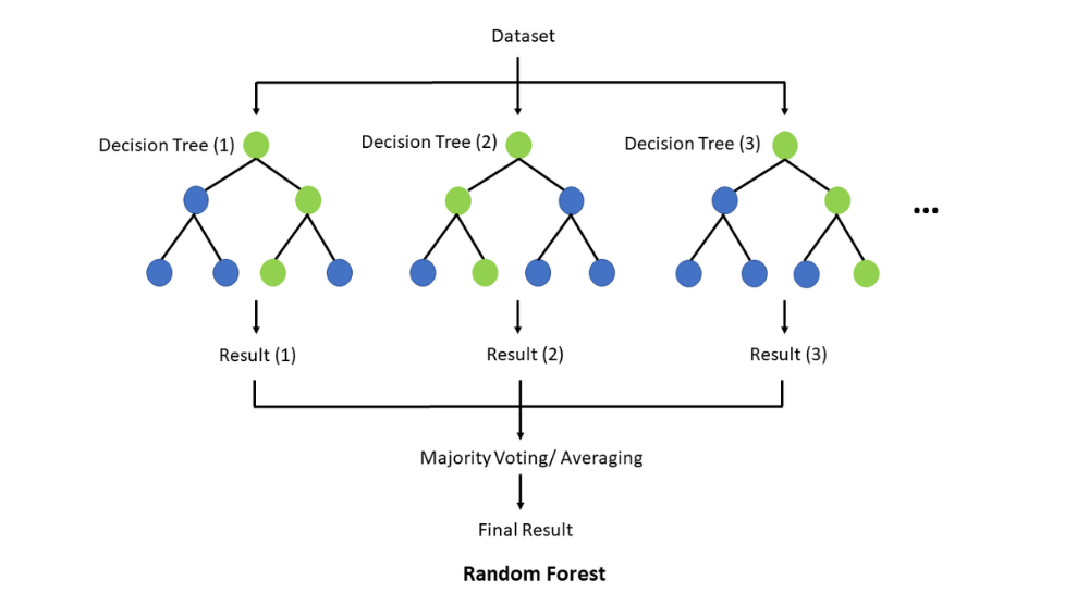
Figure 1. Basic Structure of RF Networks [6]

3.1.2. Gradient Boosting Decision Tree (GBDT). GBDT (Gradient Boosting Decision Trees) is an ensemble learning method. It is based on the decision tree model and gradient lifting algorithm and iteratively trains multiple decision trees to improve the performance of the model. Here are the basic principles of GBDT.

1. Decision Tree and Regression: The basic model of GBDT is also the decision tree. In GBDT, the goal is to fit a continuous target variable. The initial prediction of the model can choose the average value of the target variable (for the Quadratic loss function) or other suitable initial value. Then, iteratively, the GBDT learns a series of decision trees, each attempting to correct the residual (the difference between the actual value and the current model prediction) of the previous tree.

Initialize the decision tree : \( {f_{0}}(x)=argmin \sum _{i=1}^{N}l({y_{i}}, c) \)

Quadratic loss function : \( l({y_{i}},{\hat{y}_{i}})= {({y_{i}}-{\hat{y}_{i}})^{2}} \)

For each sample i = 1, 2,... N, calculate the negative gradient,

i.e. the residual: \( -[\frac{∂l({y_{i}},{\hat{y}_{i}})}{∂{\hat{y}_{i}}}]= ({y_{i}}-{\hat{y}_{i}}) \)

2. Classification: In classification problems, the goal of GBDT is to predict discrete category labels. GBDT uses a technique called gradient lifting, in which each new decision tree attempts to correct the misclassification of the previous tree. For this purpose, GBDT uses a Log-Likelihood Loss function:

\( l ({y_{i}},{\hat{y}_{i}})={y_{i}}ln{(1+{e^{-{\hat{y}_{i}}}})}+ (1-{y_{i}})ln⁡(1+{e^{ {\hat{y}_{i}}}}) \)

3. Loss function optimization: The core idea of GBDT is to optimize the loss function. In each iteration, GBDT calculates the negative gradient of the loss function and then uses the negative gradient as the training target for the next decision tree. In this way, each tree is trying to reduce the loss of the overall model, and the model is gradually approaching the optimal solution.

Take the residual obtained in the previous step as the new true value of the sample and convert the data (x_(i ),r_im) ,i=1,2,⋯,N ,as the training data for the next tree, a new regression tree is obtained f_m(x) ,The corresponding leaf node area is R_jm j = 1, 2,.. J ,Where J is the number of leaf nodes in the regression tree t .The best fit is calculated for the leaf region j = 1, 2,.. J : Where J is the number of leaf nodes in the regression tree t .

The best fit is calculated for the leaf region j = 1, 2,.. J :

\( {r_{jm}}=argmin\sum _{{x_{i}}∈{R_{jm}}}L({y_{i}},{f_{m-1}}({x_{i}})+r) \)

Iterate to get a new tree:

\( {f_{m}}(x)={f_{m-1}}(x)+\sum _{j=1}^{j}{r_{jm}}I(x∈{R_{jm}}) \)

4. Integration: The final prediction is obtained by adding the predicted values of all trees. For regression problems, these values can be added together to get the final prediction result. For classification problems, GBDT takes a similar approach but uses Softmax functions to convert scores into category probabilities.

\( f(x)= {f_{m}}(x)= {f_{0}}(x)+\sum _{m=i}^{M}\sum _{j=1}^{J}{r_{jm}}I(x∈{R_{jm}}) \)

3.1.3. XGBoost. XGBoost (eXtreme Gradient Boosting) is a machine-learning algorithm based on gradient-boosting trees. similar to the traditional GBDT algorithm. It employs decision trees as base learners (weak learners) that are ensemble into a powerful model.

1. Objective function: The objective function of XGBoost consists of two parts: training loss and regularization term. The objective function is defined as follows:

\( f=\sum _{i=1}^{n}l({y_{i}},{\hat{y}_{i}})+\sum _{k=1}^{K}Ω({f_{k}}) \)

2.Variable interpretation:

f : Objective function

\( l({y_{i}},{\hat{y}_{i}}) \) : Loss function

(3) \( \sum _{k=1}^{K}Ω({f_{k}}) \) : Tree complexity

(4) \( {\hat{y}_{i}} \) : The predicted value of sample xi

Since XGBoost is an additive model, the predicted score is the sum of the scores for each tree.

2. Regularization Terms: To control model complexity and prevent overfitting, XGBoost introduces regularization terms, including L1 regularization (Lasso) and L2 regularization (Ridge). These regularization terms help reduce the complexity of the trees and improve model generalization.

3. Tree Construction: XGBoost employs a greedy algorithm to construct trees. At each split, it evaluates all possible split points and selects the one with the maximum gain in score. The score gain typically considers both the improvement in the loss function and the contribution of regularization terms.

Learn the t tree:

\( \hat{y}_{i}^{(t)}=\sum _{k=1}^{t}{f_{k}}({x_{i}})=\hat{y}_{i}^{(t-1)}+{f_{t}}({x_{i}}) \)

4. Boosting: XGBoost follows a boosting strategy, where each new decision tree attempts to correct the residual errors of the previous one. The model iteratively generates a sequence of trees, each aiming to reduce the value of the loss function.

3.2. Method of Deep Learning

3.2.1. RNN (Recurrent Neural Network). Recurrent Neural Network (RNN) is a neural network architecture for processing sequential data. Unlike feedforward neural networks, Recurrent neural networks have connections that loop back into themselves, allowing a continuous flow of information. Thus, it is capable of handling variable-length input sequences, and the output at each time step depends on the previous state. This structure makes RNNs well-suited for continuous data such as time series data, speech, text, etc. The basic structure of RNN is shown in Figure 2.

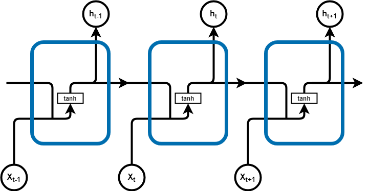
Figure 2. Basic Structure of RNN Networks

The core of an RNN is its hidden state \( {h_{t}} \) , which represents the information so far. For the input sequence \( {x_{1}},{x_{2}},… , {x_{n}} \) , the hidden state for each time step is calculated as follows:

\( {h_{t}}= σ({W_{hh}}{h_{t-1}}+{W_{xh}}{x_{t}}+{b_{h}}) \)

-h_(t-1) is the hidden state from the previous time step.

-x_t is the input of the current time step.

-W_hh and W_xhare the weight matrices.

-b_h is the deviation of the hidden state.

-σ is a nonlinear activation function such as tanh or sigmoid.

While an RNN can theoretically capture sequence dependencies of any length, in practice it often suffers from gradient vanishing and explosion problems that make it difficult for the network to learn dependencies over long distances. Gradient vanishing makes the weight updates so small that they have almost no effect, while gradient explosion makes the weight updates too large and leads to model divergence.

3.2.2. LSTM (Long-Short-Term Memory Network). Since it is often observed that its backpropagation dynamics constantly lead to gradient explosion or vanishing [7], LSTM (Long - Short-Term Memory Network) was proposed.LSTM [8] is a variant of RNN designed with special storage units to capture remote dependencies. The core idea is that by introducing three gate structures and a unit state, the network can learn when to forget old information and when to update and output new information. The basic structure of LSTM networks is shown in Figure 3.

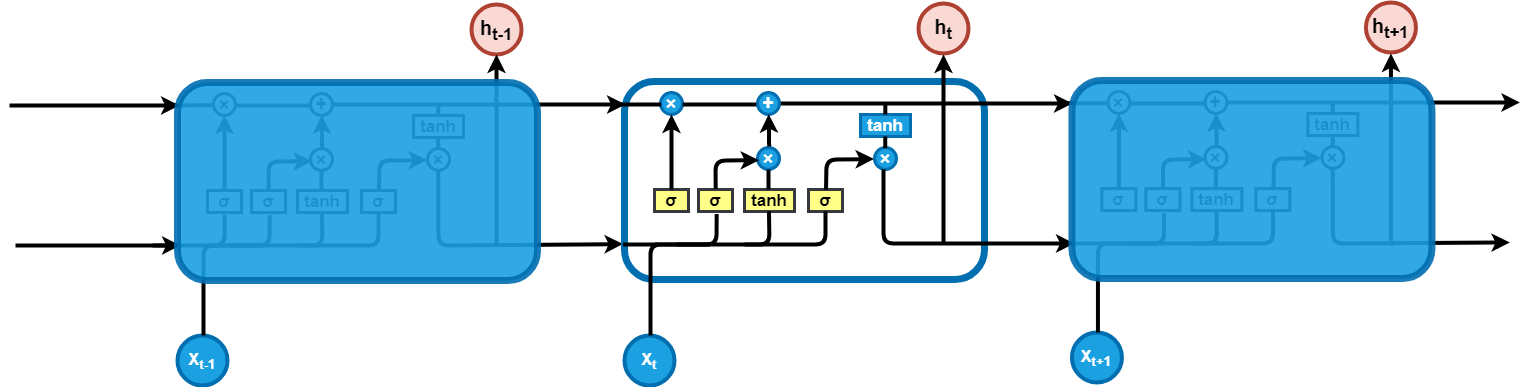
Figure 3. Basic Structure of LSTM Networks

The LSTM consists of:

Forget gate: Determines the extent to which the current time step should forget or retain the cell state of the previous time step.

\( {f_{t}}=σ({W_{f}}∙[{h_{t-1}},{x_{t}}]+{b_{f}}) \)

Input gate: Determines to what extent new input information for the current time step should be stored in the cell state.

\( {i_{t}}=σ({W_{f}}∙[{h_{t-1}},{x_{t}}]+{b_{i}}) \)

\( {\widetilde{C}_{t}}=tanh⁡({W_{f}}∙[{h_{t-1}},{x_{t}}]+{b_{C}}) \)

Update cell status: Selectively update its internal memory based on the current input and the previous state

\( {C_{t}}={f_{t}} ⨀ {C_{t-1}}+{i_{t}} ⨀ {\widetilde{C}_{t}} \)

Output gate: Decides which part of the current cell state should be passed to what extent to the hidden state of the current time step.

\( {o_{t}}= σ({W_{f}}∙[{h_{t-1}},{x_{t}}]+{b_{o}}) \)

\( {h_{t}}={o_{t}} ⨀ tanh({C_{t}}) \)

- \( {x_{t}} \) : Input at time t.

- \( {h_{t-1}} \) : the hidden state at time t-1.

- \( [{h_{t-1}},{x_{t}}] \) : the splice of the previous hidden state and the current input.

- \( {f_{t}}, {i_{t}}, {o_{t}} \) : activation of the forgetting gate, input gate and output gate at time t respectively.

- \( {C_{t}} \) : the state of the cell at time t.

- \( {\widetilde{C}_{t}} \) : the candidate cell state corresponding to the current input.

- \( {W_{f}}, {W_{i}}, {W_{o}}, {W_{C}} \) : the weight matrices of the oblivion gate, the input gate, the output gate, and the cell state, respectively, each for the spliced input .

- \( {b_{f}}, {b_{i}}, {b_{o}}, {b_{C}} \) : the bias terms for the oblivion gate, input gate, output gate and cell state, respectively.

- \( σ \) : Sigmoid activation function.

- \( tanh \) : Hyperbolic tangent activation function.

- \( ⨀ \) : Hadamard product, i.e., element-to-element product.

4. Datasets and Data Processing

Yoochoose Dataset comprises six months of user activity data for a prominent European e-commerce enterprise specializing in a wide range of consumer products, such as garden tools, toys, apparel, electronics, and more [9]. The training data consists of two distinct files: yoochoose-clicks.dat and “yoochoose-buys.dat. There was a total of 33,040,175 records in the clicks file and 1,177,769 records in the buys file. Each record in yoochoose-clicks.dat contains four key fields: Session ID, Time stamp, Item ID, and Item category. Within yoochoose-buys.dat, each record represents a purchase and contains five essential fields: Session ID, Time Stamp, Item ID, Item Price, and Quantity.

The Yoochoose Datasets [7] have been merged into one dataset after data processing. The contents include Session ID, Date, Holiday (from seven days before the holiday to the holiday itself), View Time (total browsing time for each session), Number of Clicks (number of clicks in each session), Number of View Items (number of products viewed in each session), Number of Bought Items (number of products purchased in each session).

4.1. Data Loading and Conversion

In this section, there are the steps undertaken to preprocess the raw data obtained from the Yoochoose Datasets, providing insights into the rationale behind each operation. Duplicate or empty lines were removed from the original datasets and new csv files were generated. These two files then were loaded into Pandas DataFrames. The data types for the 'Session ID' and 'Item ID' columns were specified, ensuring compatibility and efficient manipulation.

4.2. Timestamp Standardization

One critical aspect of our data preparation involved standardizing the 'Timestamp' column across both data frames. The 'Timestamp' data were converted into datetime objects to facilitate temporal analysis, which is a fundamental requirement for our research.

4.3. Holiday Identification

For context-specific analysis, a new column 'Holiday' was introduced within the cleaned ‘clicks’ data frame. The 'holidays' library was employed to identify dates corresponding to US holidays. This addition assists us in understanding user behavior patterns during holiday periods.

4.4. Temporal Window Consideration

Recognizing that user activity around holidays may extend beyond the holiday date, a 7-day window mechanism was implemented. Instances were identified when user activity occurred within a 7-day window of a holiday. This enhancement offers a more nuanced perspective on user behavior [10].

4.5. Calculation of Key Metrics

To gain deeper insights into user interactions, several key metrics were calculated. These included 'View Time' and 'Number of Clicks.' 'View Time' was derived as the time difference between the first and last timestamp within each session, providing us with a comprehensive view of user engagement. Concurrently, 'Number of Clicks' was computed to quantify user interaction intensity.

4.6. Number of Viewed Items

Understanding the diversity of user interactions is crucial. This was quantified by calculating the 'Number of Viewed Items,' capturing the unique items viewed within each session.

4.7. Number of Bought Items

The 'Number of Bought Items' is a significant metric in our research. This information was extracted by counting the unique 'Item ID' values within the cleaned 'buys' data frame. Subsequently, this data was merged with the 'clicks' data frame to enrich the dataset.

4.8. Date Extraction and Aggregation

The date of the first appearance of the 'Timestamp' within each session was captured and merged with other aggregated data. This step allowed us to analyze the relationship between the timing of user interactions and their actions.

4.9. Data Filtering and Sorting

To enhance the quality and interpretability of our dataset, data records were filtered and retained where 'View Time' ranged from 50 seconds to 100,000 seconds, removing outliers. Furthermore, the new data frame was sorted based on the 'Date' column as DateTime objects, ensuring a chronological order for temporal analysis.

4.10. Data Visualization and Outlier Handling

A scatter plot was employed to visualize the 'View Time' data, with each data point representing a session. The x-axis denotes the index of the data points, while the y-axis represents the 'View Time.' This scatter plot provided us with an initial insight into the distribution of 'View Time' across the dataset. During the data visualization phase, it became evident that the View Time in the dataset contained some extreme values, both exceedingly large and exceptionally small. These outliers can adversely affect the reliability of subsequent analyses and may not be representative of typical user behavior.

Before further data processing, the view time in each session is shown in figure 4:

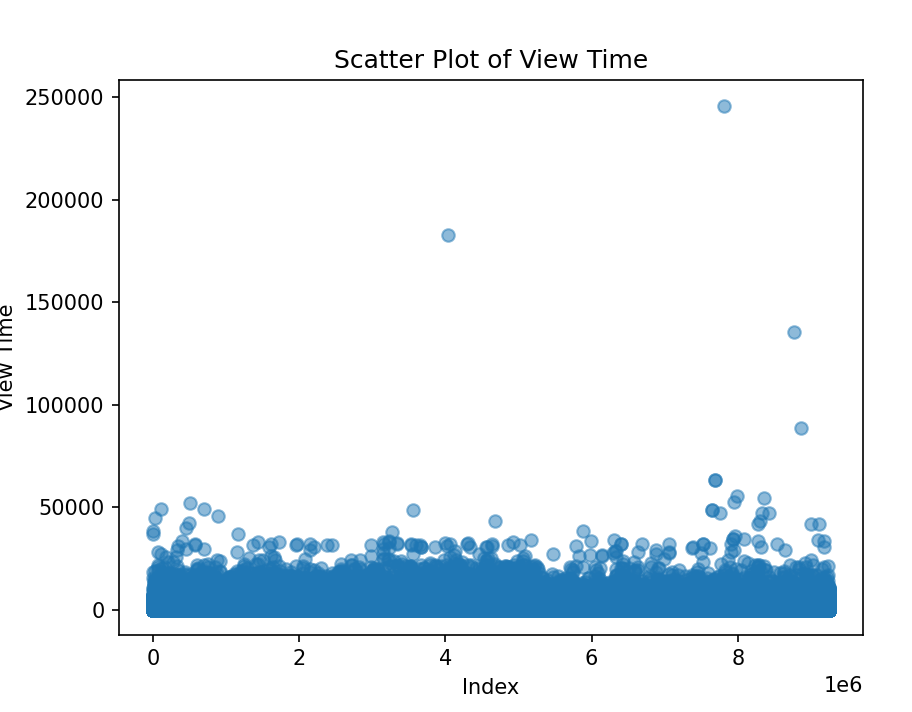
Figure 4. Scatter Plot of View Time Before Data Processing

From the chart, it can be observed that some View Times are excessively long (over 100,000 seconds), potentially lacking reference value, and could be considered for removal. For View Times that are too short (less than 50 seconds), they should also be removed to ensure more accurate experimental results.

After removing the outliers and small values, the results are shown in the following figure 5.

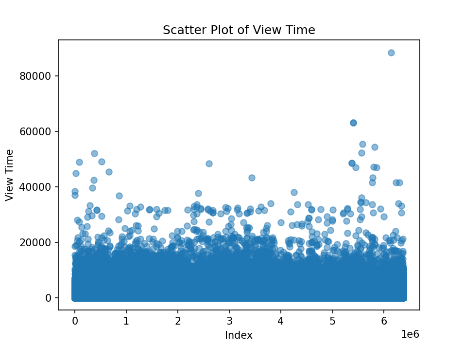
Figure 5. Scatter Plot of View Time After Data Processing

5. Exp. Settings

5.1. Machine Learning

5.1.1. Sliding time Window. The time window for the dynamic in the experiments is set from 4 to 6 days. ie. Use data from date 4.1 to 4.5 to predict purchases on 4.6, data from date 4.2 to 4.6 to predict purchases on 4.7, and so on

5.1.2. Data Pre-processing. Since there is an imbalance in the data (the ratio of buy to not buy is close to 1:9),so we need to pre-process the data. First, select a time window, extract the data belonging to this time window, separate the purchased data from the unpurchased data, and then divide the unpurchased data into 9 parts on average, and combine each of the unpurchased data with the purchased data one by one, then we will get 9 training sets

5.1.3. Training Model. In the data preprocessing, we get 9 training sets, we use machine learning once for each training set, then, we will get a total of 9 different model

5.1.4. Test and Combine the Model. We put the test set into each model and we get 9 sets of predictions. In these 9 sets of predicted values, for each sample, if there is P(x) > 0.5 (the predicted probability of successful purchase is greater than 0.5), then this sample is predicted as a successful purchase, otherwise it is predicted as no purchase.

5.1.5. Model Selecting. We Sequentially train 9 models based on different time windows (ranging from 4 to 10 days) using random forest (The number of trees in the forest is set to 100), GBDT (The maximum number of iterations of the weak learner is 100), and XGBoost (Tree model as a base classifier and the total number of iterations is 100) classifiers. Finally, we evaluate and compare the models based on their prediction accuracy on the test set.

5.2. Deep Learning

In this part, we will introduce the LSTM-based model construction and training process in detail. First, the raw data is pre-processed, including balance labeling, and data standardization. Next, we describe the structure of the complex and simple LSTM models. The main parameters used in the model training are then listed. Finally, the training and evaluation strategies of the model are described in detail.

5.2.1. Data Pre-processing. Prior to model training, we first performed a series of preprocessing operations on the raw data to ensure its effectiveness for model training. First, since there is a significant imbalance between purchased and non-purchased labels in the dataset, we divided the dataset into 13 subsets equally to ensure that the proportion of purchased and non-purchased labels is the same in each subset, thus avoiding the model being biased towards either category. Next, we extracted features about hours and days of the week from date timestamps to provide more contextual information for the model. Finally, to ensure that the model can effectively capture the relationships between features without being affected by their magnitude, we normalized all features.

5.2.2. Model Structure. To test the LSTM's performance on this task, we designed two model structures: a simple model and a complex model. The following are the main structural features of both models:

Table 1. Model comparison of the two structures

5.2.3. Parameter Setting. For both models, we used the Adam optimizer with the learning rate set to 0.01. To prevent overfitting, L2 regularization was used for the LSTM and Dense layers in the model. In addition, we set up a learning rate decrease strategy so that when the verification loss is no longer decreasing, the learning rate is reduced to 0.2 times its original value, with a minimum learning rate of 0.0001.

5.2.4. Training and Verification. Using the above parameters and structure, we trained each model for 200 epochs. To monitor the performance of the models during training, we used TensorBoard for real-time visualization and set up Receiver Operating Characteristic callbacks to monitor the Area under the ROC Curve values of the models. The training data and validation data were divided in a ratio of 8:2 and trained using a batch size of 32.

With this approach, we can ensure that training and validation are performed on 13 independent datasets to fully evaluate the performance of the model. After completing the training on all datasets, we will calculate the average AUC value as a comprehensive assessment of the model performance.

6. Exp. Result & Discussion

6.1. Machine Learning

Due to the huge amount of data, we have selected part of the results for display. Here, we choose to show the data training results from 2014/4/1 to 2014/4/11

6.1.1. Random Forest

5D time windows

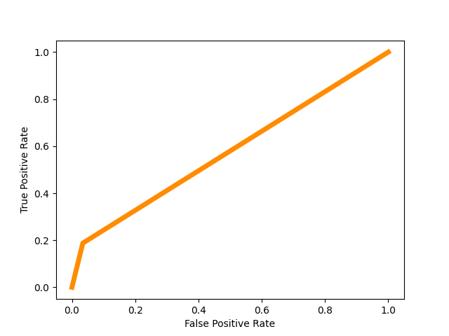
Figure 6. Confusion matrix Figure 7. Roc curve

Figure 6 shows the confusion matrix of the predicted value by using Random Forest and the true value at the date 2014/4/6

Figure 7 shows the Roc curve by using Random Forest at the date 2014/4/6

Table 2. different accuracy by using Random Forest

Table 1 shows different accuracy corresponding to conditions with different time window sizes by using Random Forest

6.1.2. GBDT

5D time windows

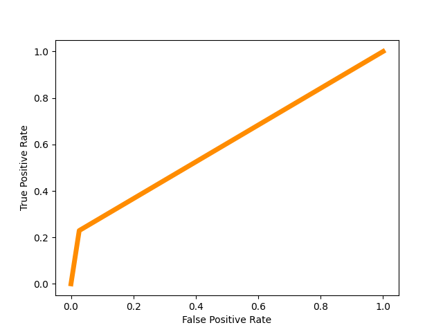
Figure 8. Confusion matrix Figure 9. Roc curve

Figure 8 shows the confusion matrix of the predicted value by using GBDT and the true value at the date 2014/4/6

Figure 9 shows the Roc curve by using GBDT at the date 2014/4/6

Table 3. different accuracy by using GBDT

Table 3 shows different accuracy corresponding to conditions with different time window sizes by using GBDT

6.1.3. XGboost

5D time windows

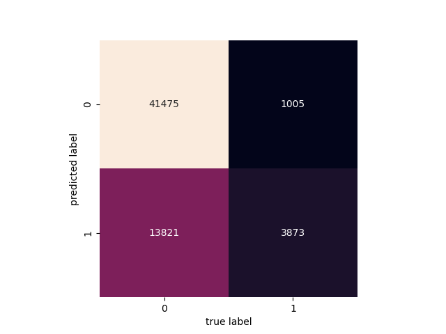
Figure 10. Confusion matrix Figure 11. Roc curve

Figure 10 shows the confusion matrix of the predicted value by using XGboost and the true value at the date 2014/4/6

Figure 11 shows the Roc curve by using XGboost at the date 2014/4/6

Table 4. Different accuracy by using XGboost

Table 4 shows different accuracy corresponding to conditions with different time window sizes by using XGboost

By looking at the results of different machine learning models running at different times in Windows, it is not difficult to see that the accuracy of the model's predictions increases as the window size increases. However, when the window size reaches 10 days, the accuracy decreases, which may cause the problem of overfitting. The prediction accuracy using GBDT and XGboost models is better than the prediction accuracy using Random Forest models

6.2. Deep Learning

We use a publicly accessible dataset as the basis for the experimental study. The dataset was processed through feature engineering, and since the proportion of "buy" and "don't buy" labels in the dataset was extremely unbalanced, we divided the original dataset into 13 equal parts, with the same proportion of "buy" and "don't buy" in each part to ensure that there were the same number of "buy" labels in each dataset. The main evaluation metrics of the model are prediction accuracy, AUC-ROC, and recall. Experiments show that our LSTM model can effectively predict customers' purchase intentions.

The formulas for prediction accuracy and recall are as follows:

\( Accuracy=\frac{Number of Correct Predictions}{Total Number of Predictions} \)

\( Recall=\frac{True Positives}{True Positives+False Negatives} \)

In these formulas, "True Positives (TP)" denotes a correct positive case, which is an instance that is itself of positive class and is also predicted by the model to be of the positive class." False Positives (FP)", on the other hand, denotes a false positive case, which is an instance that is actually a negative class but is incorrectly predicted as a positive class by the model." False Negatives (FN) "denotes a false negative situation, which is an instance of what is actually a positive class, but is incorrectly predicted by the model to be a negative class." Number of Correct Predictions" is the number of instances predicted correctly by the model, regardless of whether they are positive or negative. The "Total Number of Predictions" is the number of all predictions made by the model, whether they are correct or not.

After training 200 epochs, the average performance of the simple and complex models on 13 datasets is as follows Table 5:

Table 5. Comparison of Prediction Metrics between Simple and Complex Models

From the results, it can be observed that the simple model outperforms the complex model in both prediction accuracy and AUC-ROC. This indicates that although the complex model introduces more parameters and layers, it does not necessarily lead to better performance. The enhanced ability of the complex model to predict non-purchasing behavior may be due to the fact that the model is more inclined to predict a larger share of categories, i.e., non-purchasing behavior. In real-world applications, there is usually an imbalance between purchase and non-purchase data. Despite our processing to equalize the proportion of categories in the dataset, the model may still be affected by the original data distribution.

In response to the above observations, we can try further strategies to optimize the performance of the complex model, such as adjusting the weights of the loss function, adding an attention mechanism, etc.

7. Conclusion

We introduce an innovative approach for predicting purchase intent among customer groups by leveraging clickstream datasets to construct customer behavior models. By considering special days, view times, and items they choose, we further improve the machine learning and deep learning models and both of the models give high performance and accuracy in predicting customer behavior. In addition, we narrow down the time scale for the machine learning model to give it the highest accuracy. The three machine learning models achieve the best prediction accuracy with a time window of 10 days. For deep learning, the LSTM model reaches its highest performance with 50 layers. By comparing the results of machine learning and deep learning models, we found that there is little difference between them. This finding will provide practical and efficient guidelines for companies to solve classification problems with machine learning and deep learning models. Due to the limitations of the dataset and features we generated, with more time windows, the accuracy tends to increase but severe overfitting also takes place. In future studies, our focus will shift towards a more in-depth exploration of diverse feature sets, with an aim to amplify the accuracy of both our machine learning and deep learning models. Efforts will be concentrated on refining variables to counteract overfitting issues and determining the optimal time windows for the machine learning model. On the deep learning front, our ambitions lie in perfecting the model's architecture and configuration, thus unlocking the maximal capabilities of neural networks for capturing complex patterns within clickstream data. Our strategy will involve meticulous hyperparameter adjustments, the adoption of cutting-edge regularization methods, and experimenting with varied neural network structures, all contributing to heightened model efficiency and stability.

Acknowledgement

Deming Liu, Hansheng Huang, Haimei Zhang, Xinyu Luo and Zhongyang Fan contributed equally to this work and should be considered co-first authors.

References

[1]. Necula, S.C. Exploring the Impact of Time Spent Reading Product Information On E-Commerce Websites: A Machine Learning Approach to Analyze Consumer Behavior. Behav. Sci. 2023, 13, 439
[2]. Romov, P. and Sokolov, E. RecSys Challenge 2015: ensemble learning with categorical features. ACM Digital Library 2015 https://doi.org/10.1145/2813448.2813510
[3]. Sheuk, H. , Rana,O. , and Reilly, R. Predicting purchasing intent: Automatic Feature Learning using Recurrent Neural Networks. SIGIR 2018 eCom, July 2018, Ann Arbor, Michigan, USA
[4]. Sakar, C.O., Polat, S.O. Katircioglu, M., and Kastro, Y. Real-time prediction of online shoppers’ purchasing intention using multilayer perceptron and LSTM recurrent neural networks. Neural Comput. Appl. 2019, 31,6893–6908
[5]. Piao,Q., Lee,J.Y., and Sakai,T. , ‘Purchase Prediction based on Recurrent Neural Networks with an Emphasis on Recent User Activities’. Available online: https://proceedings-of-deim.github.io/DEIM2020/papers/B4-3.pdf
[6]. Wikipedia contributors. (n.d.). Random forest [Figure]. In Wikipedia. Retrieved from https://de.wikipedia.org/wiki/Random_Forest
[7]. Pascanu,R. , Mikolov,T. , and Bengio,Y. , ‘On the difficulty of training Recurrent Neural Networks’. arXiv, Feb. 15, 2013. Accessed: Sep. 30, 2023. [Online]. Available: http://arxiv.org/abs/1211.5063
[8]. Hochreiter,S. and Schmidhuber,J., Long Short-Term Memory, Neural Computation, vol. 9, no. 8, pp. 1735–1780, Nov. 1997, doi: 10.1162/neco.1997.9.8.1735.
[9]. Shimon, B.D. Tsikinovsky, A. ,and Friedmann, M. RecSys Challenge 2015 and the YOOCHOOSE Database. ACM Digital Library 2015. https://doi.org/10.1145/2792838.2798723
[10]. G. Sılahtaroğlu and H. Dönertaşli, Analysis and prediction of Ε-customers' behavior by mining clickstream data, 2015 IEEE International Conference on Big Data (Big Data), Santa Clara, CA, USA, 2015, pp. 1466-1472, doi: 10.1109/BigData.2015.7363908. https://ieeexplore.ieee.org/document/7363908
Cite this article
Liu,D.;Huang,H.;Zhang,H.;Luo,X.;Fan,Z. (2024). Enhancing customer behavior prediction in e-commerce: A comparative analysis of machine learning and deep learning models. Applied and Computational Engineering,55,181-195.
Data availability
The datasets used and/or analyzed during the current study will be available from the authors upon reasonable request.
Disclaimer/Publisher's Note
The statements, opinions and data contained in all publications are solely those of the individual author(s) and contributor(s) and not of EWA Publishing and/or the editor(s). EWA Publishing and/or the editor(s) disclaim responsibility for any injury to people or property resulting from any ideas, methods, instructions or products referred to in the content.
About volume
Volume title: Proceedings of the 4th International Conference on Signal Processing and Machine Learning
© 2024 by the author(s). Licensee EWA Publishing, Oxford, UK. This article is an open access article distributed under the terms and
conditions of the Creative Commons Attribution (CC BY) license. Authors who
publish this series agree to the following terms:
1. Authors retain copyright and grant the series right of first publication with the work simultaneously licensed under a Creative Commons
Attribution License that allows others to share the work with an acknowledgment of the work's authorship and initial publication in this
series.
2. Authors are able to enter into separate, additional contractual arrangements for the non-exclusive distribution of the series's published
version of the work (e.g., post it to an institutional repository or publish it in a book), with an acknowledgment of its initial
publication in this series.
3. Authors are permitted and encouraged to post their work online (e.g., in institutional repositories or on their website) prior to and
during the submission process, as it can lead to productive exchanges, as well as earlier and greater citation of published work (See
Open access policy for details).