1. Introduction

Functional Magnetic Resonance Imaging, short for fMRI, measures and maps brain activation by detecting blood-oxygen-level-dependent (BOLD) signals [1]. The BOLD signal reflects the concentration of oxygen change in hemoglobin in brain blood flow since more blood flow is needed in activated areas. This technique helps to examine the activated area when processing specific projects and actions, determine the critical function of each site, evaluate brain diseases, and guide brain treatment. Statistical Parametric Mapping (SPM) is a MATLAB tool to examine people's brain activity differences by model fitting and statistical analysis [1]. fMRI datasets contain concatenated strings of volumes a run of data. The signal measured in the volumes of the entire run is a time series. After processing the datasets and fitting the model, the result is used to do the statistical analysis. The statistical analysis is closely related to the gamma distribution because of the characteristics of the BOLD signal, which are consistent shape and the bell curve. When a BOLD signal tries to fit in the gamma distribution, it has a new name: canonical Hemodynamic Response function, or HRF [1]. Another critical theory is the general linear model (GLM), which is the basis of SPM [1]. However, specific objections exist to using this model to calculate the BOLD signal, such as the assumption of linearity. After using SPM on Flanker tasks, the apparent activation should be spotted on the prefrontal and anterior cingulate cortex regions because Flanker tasks are the same assignments, which require looking and making decisions [2]. In Flanker tasks, under incongruent conditions, if most of the arrows are pointing to the right, but there is only one arrow pointing to the left, then the subject presses the left button [1]. Vice versa, if all the arrows indicate to the right, the subject will press the “right” button. Overall, the task would be more straightforward and accurate if all the arrows point in the same direction. Flanker tasks aim to find the difference between congruent and incongruent conditions.

2. Method

2.1. Downloading and Installing SPM

The Andy’s Brain Book website has the link to download the latest SPM file, spm12. After typing in “spm fmri” in MATLAB, downloading the Data becomes the next step.

2.2. Downloading the Data

Flanker tasks are the group of data that needs to be analyzed by SPM fMRI. This group of data is provided on the “OpenNeuro” website. After clicking on the link, the download button is available.

2.3. Looking at the Data

The file has 26 data groups collected from individuals with the same tasks. After downloading the data on the computer, use the SPM Graphical User Interface to check every subject's anatomical and functional images for artifacts. This step also ensures that each image is positioned for future operations.

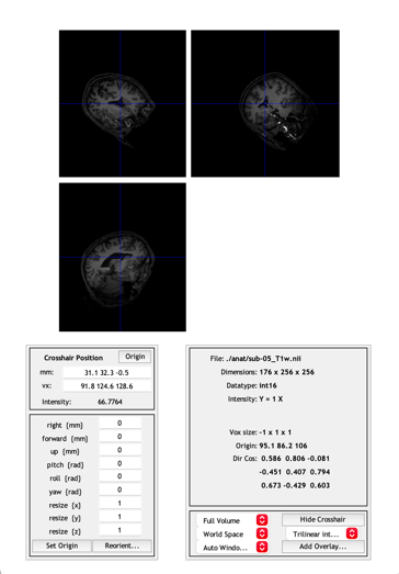
Figure 1. The display of the anatomical image in Subject 5

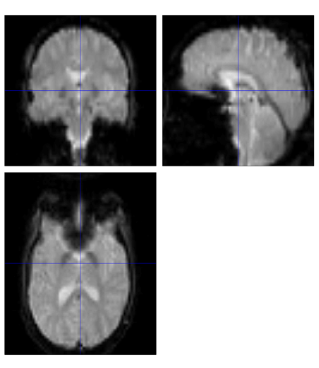
Figure 2. The Functional image of run-1 in Subject 5

2.4. Preprocessing

This whole step can clean up the images and place the image onto the same template to be ready to compare under different conditions.

2.4.1. Realigning and Unwarping the Data

Click this step's “Realign (Estimate & Reslice)” button. Estimate means estimating the out-of-realignment with a reference volume. Reslice means aligning all the volumes with the reference volume (Andy’s Brain Book) [1].

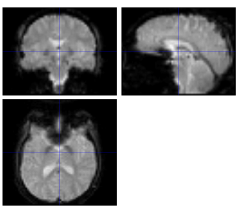
Figure 3. The Functional image of run-1 in Subject 5 after Realign step

2.4.2. Slice-Timing Correction

Click on the “Slice Timing” button in this step. Like these words, this step is to slice the image into many slices. There are two typical slice ways. One is the sequential slice acquisition, which either cuts from bottom to top or from top to bottom. Another one is interleaved slice acquisition, which acquires every other piece. However, there are some objections. First, with short TRs, the slice-timing correction does not play any role. Second, the temporal derivative in the statistical model could substitute the slice-timing correction.

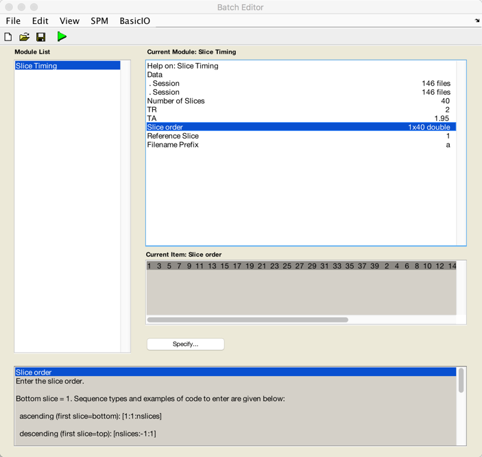
Figure 4. The panel of “Slice Timing” with two functional images input as the session of Subject 5

2.4.3. Coregistration

Click on this step's “Coregister (Estimate & Reslice)” button. In this step, Registering and normalizing to a template happen on the image to fit them in the same size, shape, and dimensions by a linear transformation containing four types: translation, rotation, zooms, and shears. However, this is the step that could easily produce errors. The images could easily be warped unproperly during zooming in and out and shearing.

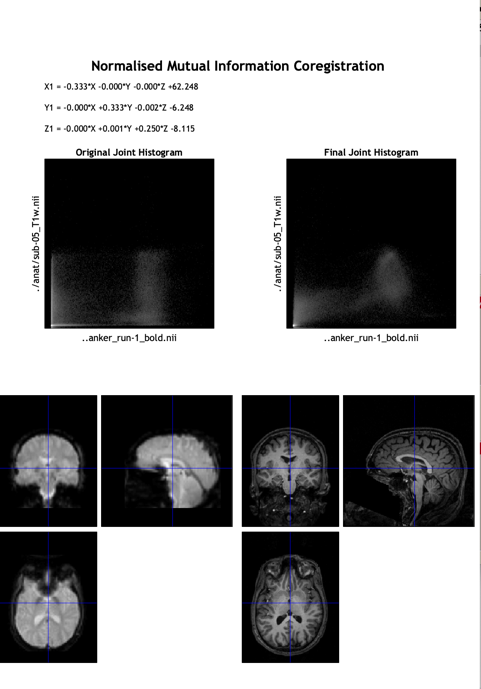
Figure 5. The screenshot of the graphic report after the Coregistration of Subject 5

2.4.4. Segmentation

Click on the “Segmentation” button for this step. Warp the image to a template in a standardized space to know which voxel belongs to which tissue type, locating the brain area and activation signal more quickly.

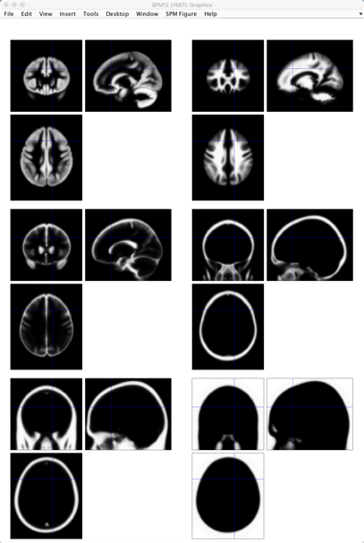
Figure 6. The graph of Segmentation of Subject 8 from Andy’s Brain Book

The upper two tissue types are grey matter and white matter. Grey matter contains a high concentration of neuronal cell bodies. White matter contains nerve fibers. The middle two are cerebrospinal fluid (CSF) and the skull. Cerebrospinal fluid is mainly located within the brain called ventricles. The lower two are the soft tissue and the air inside the sinuses and outside the brain. Showing the map of the air inside could contribute to detecting abnormal tissue, such as tumors, starting a solid effect in the clinical area.

2.4.5. Normalization

Click on “Normalize (Write)” for this step. Normalizing the image to the standard graph helps to progress in the statistical analysis steps.

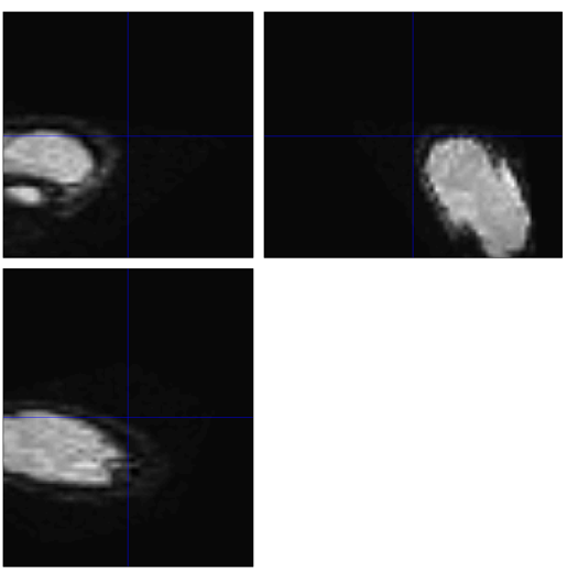
Figure 7. The screenshot of the functional image of run-1 in Subject 5 after Normalization

Here, the error occurs after the Normalization step. In this graph, the brain is not even in its appropriate spot, affecting the following steps and statistical analysis afterward. This error also might be caused by the last step – Segmentation.

2.4.6. Smoothing

The last step of preprocessing data is Smoothing. Click “Smooth” for this step. Smoothing the image or replacing the signal at each voxel with a weighted average of the voxel's neighbors eliminates the noise, affecting the proper performance of standard signals. Even though this step would decrease the resolution, the benefit outweighs the consequence.

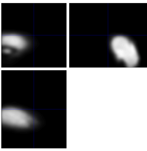
Figure 8. The screenshot of the Smoothing image of run-1 functional image in Subject 5

This step does not occur in error. The inappropriate position might be from the last two steps.

2.5. Statistics and Modeling

Next is to put all the processed data in the first-level analysis.

2.6. Creating Timing Files

In this step, type in “convertOnsetTimes” after downloading the file from GitHub and putting the file with all the subjects. Then, it will conduct all the congruent and incongruent files in each subject, later used for the first-level analysis.

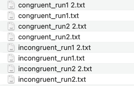
Figure 9. The screenshot of congruent and incongruent files in Subject 5 after creating the timing files step.

2.7. Running the First-Level Analysis

Click on the “Specify 1^st-Level” button for this step. This step result indicates the correlation between the ideal and actual time series. Then, the HRF, represented by beta weight, will plug into the t-test to conduct the final result of the first-level analysis.

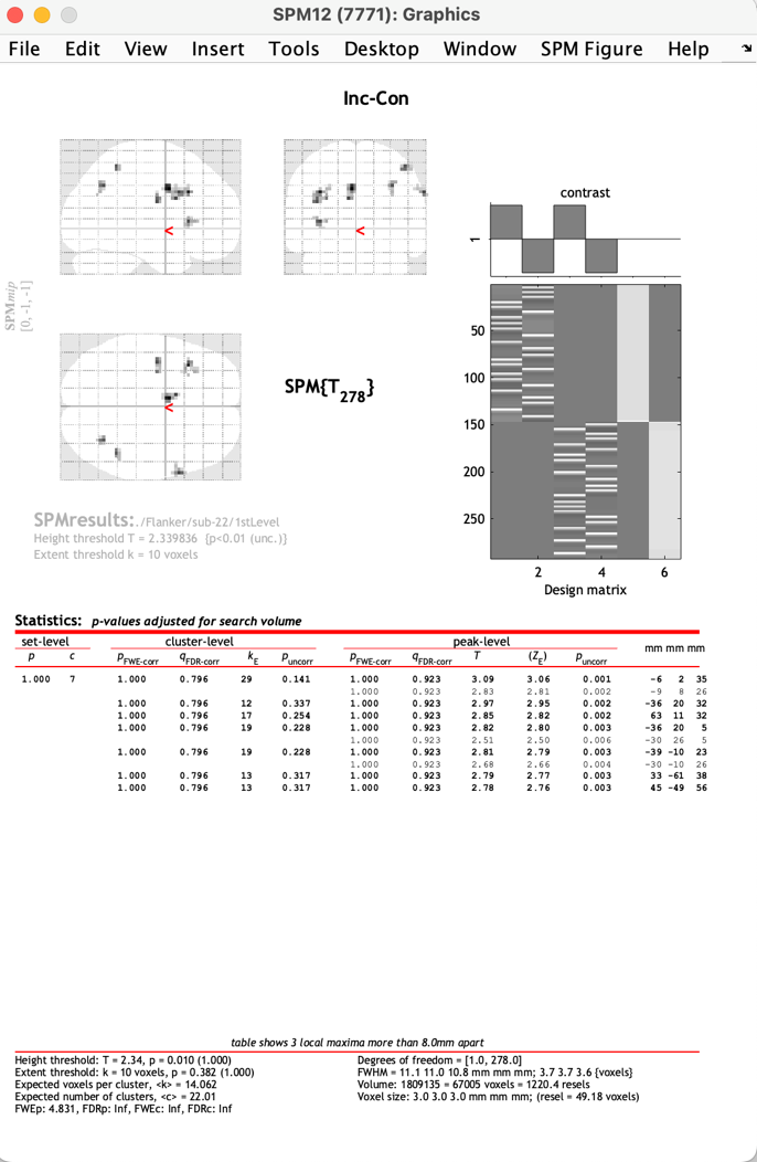
Figure 10. The report of the first-level analysis of Subject 22

On the up-right side, the lower rectangle shows the ideal time series (the first two columns), the actual time series (the middle two columns), and baseline regressors. On the up-left side, the image shows the activated spots during Flanker Tasks. At the bottom of this page, the data is listed.

2.8. Scripting

This step is putting all processes together and running with a script to simultaneously process the rest of all 26 subjects. Nevertheless, this step has two huge disadvantages. First, after processing all the subjects, it is still essential to check all the datasets. Second, it is highly possible to conduct wrong images for most subjects. Therefore, using the scripting method to save time takes colossal risks and may need to redo all the subjects.

2.9. Setting the Origin

Checking the image of every scripted graph could prevent future errors in the first-level analysis. If the image center is distributed incorrectly, this step is to readjust the center of the image and ensure the second-level analysis.

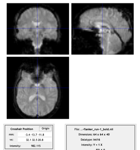
Figure 11. The screenshot after moving the origin for Subject 5

2.10. Group Analysis

Click on the button “Specify 2^nd-Level” for this step. When putting all the files from the first-level analysis and building a new t-contrast of Incongruent-Congruent, set all the weights to 1 for all 26 subjects. The resulting image will show a significant cluster representing the brain's activation with the insensitivity.

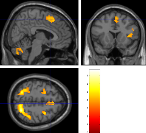
Figure 12. The image of the second-level analysis of Subject 8 from Andy’s Brain Book

2.11. ROI Analysis

ROI analysis, also known as the region of interest” helps to locate where the activation exactly is. This could provide the focus for scientists who do not have an idea of their research area of the brain. Furthermore, the spherical ROI could continue to help us focus on the area of the brain.

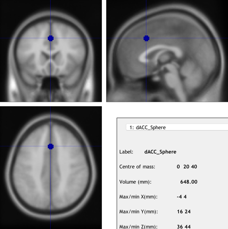
Figure 13. The image of ROI created by Marsbar from Andy’s Brain Book

3. Conclusion

There are four speculations about the incorrect result from processing the Flanker Task.

The first possibility would occur on the previous check of 26 data groups. When checking all the 26 data, there might be ignorance of the position of each brain image. This would cause a shift when cutting the brain image onto the template. Consequently, the improper detection of brain activities would occur.

Second, GLM behind the SPM could cause the error. When applying the general linear model, four assumptions must be met: linearity, homoskedasticity, normality, and independence. These assumptions can cause huge mistakes. When creating a linear function, the outliers with high leverage would have a considerable influence, making the whole function farther away from its real mean. When applying a general linear model to the data, homoskedasticity is one error aspect to consider. Homoskedasticity requires the existence of a group of constant variances. However, too many data groups in this task lead to multiple variances, and then the model becomes not well-defined. The third thing the GLM assumes is normality. Normality in GLM means the response variables are normally distributed. Just as the previous assumption, the response variables are not necessarily normally distributed. The fourth assumption is independence. Dependent variables relate to the independent variables. There is no such test to see if the variable in the fMRI function is independently associated with each other before applying this assumption to it. These data might not be independent due to the role of the whole brain. A simple procedure would need the cooperation of several parts of the brain. On another aspect, other than the bias that is created from those assumptions of GLM, the variance of the estimators, power and false positive rate are also could be the key elements of the problem [3].

Third, every time statistical analysis applies, whether this test is biased is a critical question. “Puzzlingly High Correlations in fMRI Studies” pointed out that some correlations in imaging studies were inflated because of “Nonindependence” or “Circular Analysis” (Andy’s Brain Book). “Nonindependence” means the collaboration in the brain parts since one simple action needs several functions [4]. For example, laughing needs the work of emotional sensors, the movement of the facial muscle, and possibly the vibration of the vocal cords. Circular Analysis indicates that when choosing the subject of the brain, it is possible to identify the region of the brain that is related to the function without being the primary center responsible for this function [2]. However, this mistake could bring errors because only a specific brain is needed and recorded. Also, circular analysis would exaggerate the influence of noise during the experiment time. The abnormal signals may look like standard brain activation signals during the data collection. In addition, the circular analysis would use the same database twice. Then, it may amplify the intensity of specific movements, graphing the tiny signals on the brain graph.

The fourth assumption is that the biased ROI could lead to an Inflated Effect Size. When setting the threshold, the noise could be the only thing passing the entry in that area, which leads to a more significant effect size. When adjusting the threshold, some noise signals may occur on the map because some processes could exaggerate the disturbance to make it a qualified sign. In some exceptional cases, the result would still be the same even if the threshold is up a bit. However, the result should differ from some areas' signal intensity. On another aspect, more data would also prevent the bias from occurring. The baseline of the amount of data would be 50, but in this assignment, there are barely 26 data groups.

How to create unbiased ROIs is crucial. There are three solutions. First, create unbiased ROIs from an atlas, a map that partitions the brain into anatomically distinct regions [1]. A precise version of the brain helps the distinction of brain activation regions. Second, creating a sphere centered at the coordinates reported by another study would lead to unbiased ROIs [1]. This combines the data to a different coordinate not explicitly designed for this data group. It could eliminate some of the bias with unbiased coordinates. Third, unbiased ROIs can be created by plugging in vast data. It would provide a solid amount of data for the data analysis in this process. Enough data helps to eliminate errors and bias during statistical procedures. ROIs cannot be unbiased, but they can lessen the biased effect.

Since many possible errors would occur during the process of conducting a brain activation map result, the updating of the analyzing method becomes urgent. During the statistical analysis process, the model selection is crucial. In the SPM function, the general linear model has high demands on data sets, but data should be random to ensure fairness. Bias would be another huge aspect when considering the mistake of the processing system. Bias only can be as small as possible by importing more data into the analysis model. It cannot disappear from the data model. None of the models should be extremely accurate from ideal calculation.

Overall, there are many possible areas during the analyzing process for the error to occur. The occurrence of some error and bias is non-avoidable practically and theoretically. Other than this research program, “bias also can occur in the planning, data collection, analysis, and publication phases of research” [5]. A solid, extensive database is always the best approach to eliminate mistakes.

Acknowledgments

Thanks to Professor Chunlei Liu for helping to teach me knowledge. Thanks, TA Yuan, for giving instructions on SPM and Flanker tasks. Thanks, my teammates, for dealing with the data together and getting familiar with strange software.

References

[1]. SPM Overview, Andy’s Brain Book, https://andysbrainbook.readthedocs.io/en/latest/SPM/SPM_Short_Course/SPM_fMRI_Intro.html
[2]. Kriegeskorte, Nikolaus et al. “Everything you never wanted to know about circular analysis, but were afraid to ask.” Journal of cerebral blood flow and metabolism: official journal of the International Society of Cerebral Blood Flow and Metabolism vol. 30,9 (2010): 1551-7. doi:10.1038/jcbfm.2010.86
[3]. Eriksen & Eriksen, 1974, “Eriksen flanker task”, https://www.sciencedirect.com/topics/neuroscience/eriksen-flanker-task
[4]. Martin M. Monti. March, 18, 2011. “Statistical Analysis of fMRI time-series: a critical review of the GLM approach.” Doi: 10.3389/fnhum.2011.00028
[5]. Pannucci, Christopher J, and Edwin G Wilkins. “Identifying and avoiding bias in research.” Plastic and reconstructive surgery vol. 126,2 (2010): 619-625. doi:10.1097/PRS.0b013e3181de24bc
Cite this article
Ning,K. (2024). Four possible error conjectures with SPM in MATLAB. Applied and Computational Engineering,55,196-205.
Data availability
The datasets used and/or analyzed during the current study will be available from the authors upon reasonable request.
Disclaimer/Publisher's Note
The statements, opinions and data contained in all publications are solely those of the individual author(s) and contributor(s) and not of EWA Publishing and/or the editor(s). EWA Publishing and/or the editor(s) disclaim responsibility for any injury to people or property resulting from any ideas, methods, instructions or products referred to in the content.
About volume
Volume title: Proceedings of the 4th International Conference on Signal Processing and Machine Learning
© 2024 by the author(s). Licensee EWA Publishing, Oxford, UK. This article is an open access article distributed under the terms and
conditions of the Creative Commons Attribution (CC BY) license. Authors who
publish this series agree to the following terms:
1. Authors retain copyright and grant the series right of first publication with the work simultaneously licensed under a Creative Commons
Attribution License that allows others to share the work with an acknowledgment of the work's authorship and initial publication in this
series.
2. Authors are able to enter into separate, additional contractual arrangements for the non-exclusive distribution of the series's published
version of the work (e.g., post it to an institutional repository or publish it in a book), with an acknowledgment of its initial
publication in this series.
3. Authors are permitted and encouraged to post their work online (e.g., in institutional repositories or on their website) prior to and
during the submission process, as it can lead to productive exchanges, as well as earlier and greater citation of published work (See
Open access policy for details).