1. Introduction

With the rapid development of information technology and the widespread use of smart devices, smart pens have emerged as a convenient and efficient input tool, gradually demonstrating their unique advantages in fields such as education, office work, and artistic creation. Smart pens not only fulfill the functions of traditional writing instruments but also utilize digital methods to record, store, and transmit written content, significantly enhancing users' writing experience and data processing capabilities.

Currently, smart pens on the market primarily rely on technologies such as camara [1,2], pressure sensing [3], capacitive sensing, and optical recognition. Although these technologies have achieved some success in practical applications, they also have limitations. For instance, pressure sensors can wear out after prolonged use, leading to decreased measurement accuracy; capacitive sensing technology struggles with multi-touch and complex gesture recognition; and optical recognition technology is easily affected by external lighting, impacting recognition performance. Therefore, finding a more stable and efficient smart pen design has become a focal point of research.

Vector magnetic sensing technology, as an emerging sensing technology, has shown promising application prospects in the field of smart devices in recent years. In 2010, Yang et al. combined particle swarm optimization with the Levenberg-Marquardt (LM) algorithm to achieve the positioning and tracking of three magnetic dipole targets [4]. In 2018, Gao et al. applied the LM algorithm for locating moving magnetic targets [5]. Vector magnetic sensors can detect the strength and direction of magnetic fields and convert this information into precise spatial position and orientation data through algorithms. Compared to traditional sensing technologies, vector magnetic sensing offers high sensitivity, strong anti-interference capability, and good stability, making it particularly suitable for application in smart pen design.

This paper aims to explore the design of smart pens based on vector magnetic sensing technology. By analyzing its working principles, key technologies, and application scenarios, we will verify its feasibility and advantages in practical applications. First, we will introduce the basic principles and characteristics of vector magnetic sensors; then, we will detail the system design and hardware implementation of the smart pen; next, we will analyze the software algorithms and data processing methods; finally, we will validate the performance of the smart pen through experiments and practical applications, while also looking ahead to its future development directions.

2. Mathematical Model of Magnetic Positioning Methods

Between 1820 and 1821, J. B. Biot and F. Savart conducted experiments on straight electric currents and electromagnetic forces. They concluded that the electromagnetic force exerted on a point at a distance d from a straight conductor is directly proportional to the current intensity I and inversely proportional to the distance d. This is known as the Biot-Savart Law, and the magnetic positioning studied in this article is based on this principle.

2.1. Biot-Savart Law

As shown in Figure 1, the current element dl has a current intensity of I, point P is any observation point, r is the distance between the current element and point P, and θ is the angle between the line connecting the current element to observation point P and the current element itself. The direction of the magnetic flux density dB generated by the current element at point P can be determined using the right-hand rule of Ampère; at point P, the magnetic flux density direction is perpendicular to the paper and directed inward. The magnitude of the magnetic flux density dB can be obtained using the Biot-Savart law, as indicated in equation (1). The vector form of the Biot-Savart law can be found in equation (2). \( {μ_{0}} \) is the magnetic permeability of free space.

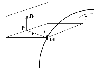
\( |dB|=\frac{{μ_{0}}}{4π}\frac{I|dl|sin{θ}}{{|r|^{2}}}\ \ \ \ \ \ （1） \)

\( dB=\frac{{μ_{0}}}{4π}\frac{Idl×r}{{|r|^{3}}}\ \ \ （2） \)

2.2. Magnetic Dipole Localization Model

The magnetic field generated around ferromagnetic targets, together with the background magnetic field, causes a distortion in the surrounding magnetic field, known as magnetic anomaly. When the detection distance exceeds three times the size of the target, it can be treated as a magnetic dipole, with its vector magnetic field represented by Equation (3), where m denotes the target's magnetic moment.

\( B(m,r)=\frac{{μ_{0}}}{4π}[\frac{3(m\cdot r)r}{{|r|^{5}}}-\frac{m}{{|r|^{3}}}]\ \ \ (3) \)

2.3. Application of the L-M Algorithm to Solve the Magnetic Dipole Model

The mathematical expression for a magnetic dipole is a high-order nonlinear equation with a very complex form. Although there are currently many optimization algorithms available for solving high-order nonlinear equations, such as Powell’s method [6], Downhill Simplex [7], DIRECT [8], and multipole coordinate search methods [9], we ultimately chose the L-M (Levenberg-Marquardt) algorithm [10] as the primary method for solving the magnetic dipole model.

The L-M algorithm is an iterative method used to find the minimum of nonlinear multivariable real functions in the form of sums of squares. It has become a standard solution for nonlinear least squares problems, combining both the gradient descent method and the Gauss-Newton method. The algorithm inherits the local convergence properties of the Gauss-Newton method while also retaining the global characteristics of gradient descent. Because the L-M algorithm utilizes approximations of second-order derivative information, it is significantly faster than gradient-based methods. Essentially, it functions as a second-order gradient method, offering rapid convergence that meets real-time requirements. When the solution obtained using the L-M algorithm differs greatly from the correct solution, the algorithm behaves similarly to gradient descent, resulting in slow convergence but ensuring eventual convergence. Conversely, when the solution is close to the correct answer, the L-M algorithm operates as the Gauss-Newton method.

If m groups of magnetic field data are collected, substituting them into equation (3) will yield a nonlinear system of equations consisting of m equations, as shown in equation (4).

\( … \\ {f_{i}}(P)={B_{i}}-\frac{{μ_{0}}}{4π}\lbrace \frac{3(m\cdot r)r}{{|r|^{5}}}-\frac{m}{{|r|^{3}}}\rbrace =0 \\ {f_{i+1}}(P)={B_{i+1}}-\frac{{μ_{0}}}{4π}\lbrace \frac{3(m\cdot r)r}{|{r|^{5}}}-\frac{m}{|{r|^{3}}}\rbrace =0 \\ {f_{i+2}}(P)={B_{i+2}}-\frac{{μ_{0}}}{4π}\lbrace \frac{3(m\cdot r)r}{{|r|^{5}}}-\frac{m}{{|r|^{3}}}\rbrace =0 \\ …\ \ \ （4） \)

In Equation (4), \( r=(x-a)i+(y-b)j+(z-c)k \) represents the displacement vector between the permanent magnet and observation point P, while \( m=ni+pj+qk \) denotes the magnetic moment of the permanent magnet. B_i indicates the magnetic field strength data collected during the i-th measurement. Equation (4) can be succinctly expressed as Equation (5).

\( {f_{i}}(P)=0, i = 1, 2,..., m\ \ \ (5) \)

In equation (5), \( P=(a,b,c,n,p,q) \) ^T represents the unknown parameters, which include the position of the permanent magnet \( (a, b, c) \) and the magnetic dipole moment \( (n, p, q) \) .

Solving a system of nonlinear equations can be equivalent to an unconstrained optimization problem, where a target function is constructed to find its optimal solution (or minimum point) within the domain of the independent variables. If the target function consists of the sum of squares of several functions, then the problem of finding its minimum value is referred to as a nonlinear least squares problem.

From equation (5), it can be seen that \( f : D⊂{R^{6}}→{R^{m}} \) , \( f={({f_{1}},{f_{2}},…,{f_{m}})^{T}} \) . The definition of the objective function is provided in equation (6).

\( φ(P)=\frac{1}{2}{f(P)^{T}}f(P)\ \ \ (6) \)

Clearly, if \( φ : D⊂{R^{6}}→{R^{1}} \) , solving the system of equations (5) is transformed into the problem of finding the optimal solution (or minimum point) for expression (6). This is a nonlinear least squares problem, as indicated in expression (7). We will solve this problem with the L-M algorithm.

\( \underset{x∈D}{min}φ(P)=\underset{x∈D}{min}\frac{1}{2}f{(P)^{T}}f(P)\ \ \ (7) \)

3. Magnetic Sensor Error Analysis

In an ideal scenario, the measurements from the magnetic sensor are completely accurate. Depending on the position of the magnetic sensor, the three-axis readings reflect the projection of the geomagnetic field strength across the three axes, satisfying equations (8) and (9):

\( h=[{h_{x}}, {h_{y}}, {h_{z}}]\ \ \ （8） \)

\( h_{x}^{2}+h_{y}^{2}+h_{z}^{2}={|B|^{2}}\ \ \ （9） \)

B is the geomagnetic induction intensity vector, and h represents its three components.

For magnetic sensors, errors can be divided into two parts. One part originates from internal factors, including variations in three-axis sensitivity, non-orthogonality of the three axes, and zero bias. The other part comes from external sources, namely hard magnetic interference and soft magnetic interference.

The internal errors are illustrated in the figure below. Hard magnetic interference is caused by permanent magnets near the sensor, while soft magnetic interference affects both the strength and direction of the original magnetic field.

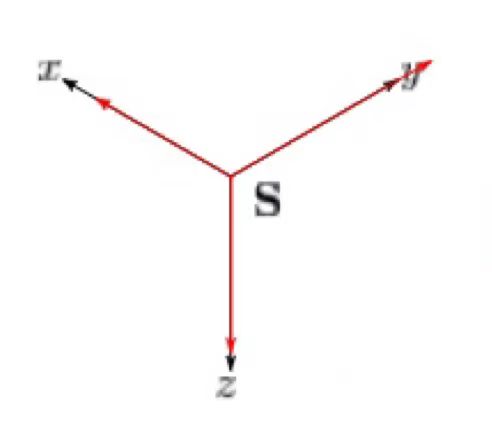
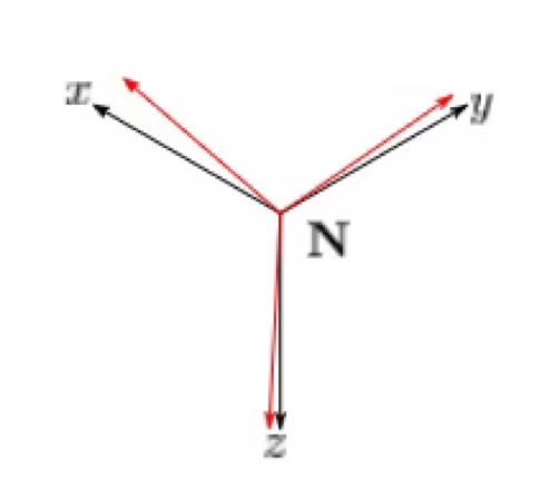
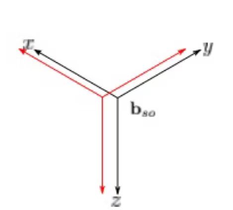
Figure 2. The internal errors.

First, the external magnetic field has been altered due to interference from both soft and hard magnetism. Consider the external interference as shown in Equation (10)

\( {h_{m}}={I_{3×3}}{h_{0}}+{F_{h}}\ \ \ (10) \)

\( {h_{0}} \) is the ideal measurement result, \( {I_{3×3}} \) is a 3 \( × \) 3 matrix representing soft magnetic interference, and \( {F_{h}} \) is a \( 3×1 \) vector representing hard magnetic interference. After considering the internal errors, we arrive at Equation (11).

\( h={S_{3×3}}{N_{3×3}}{h_{m}}+{F​_{os}}={S_{3×3}}​{N_{3×3}}({I_{3×3}}{h_{0}}+{F_{h}})+{F​_{os}}\ \ \ （11） \)

In the equation, \( {S_{3×3}} \) and \( {N_{3×3}} \) are both \( 3×3 \) matrices representing sensitivity differences and non-orthogonal effects, while \( {F​_{os}} \) is a \( 3×1 \) vector indicating zero offset.

The simplification yields the relationship between the true value and the measured value (12).

\( {h_{0}}={W^{-1}}(h-V)\ \ \ （12） \)

\( W \) is a \( 3×3 \) matrix and is symmetric, resulting in only 6 coefficients. \( V \) is a \( 3×1 \) vector, which has a total of 9 coefficients. If we only consider hard magnetic interference, then we have \( {h_{0}}=h-V \) . Since \( {h_{0}} \) lies on the sphere, there is equation (13).

\( {{h_{0}}^{T}}{h_{0}}={(h-V)^{T}}(h-V)={|B|^{2}}\ \ \ (13) \)

Both \( h \) and \( V \) can be expressed in the form of \( 3×1 \) vectors, leading to equation (14).

\( [{{h_{x}}^{2}}+{{h_{y}}^{2}}+{{h_{z}}^{2}}]-[{h_{x}} {h_{y}} {h_{z}} 1][\begin{matrix}2{V_{x}} \\ 2{V_{y}} \\ \begin{matrix}2{V_{z}} \\ {B^{2}}-({{V_{x}}^{2}}+{{V_{y}}^{2}}+{{V_{z}}^{2}}) \\ \end{matrix} \\ \end{matrix}]\ \ \ (14) \)

For the above equation, we can use the least squares method to determine the bias value.

4. Smart Pen Assistant App Design

We have obtained the equations regarding magnetic moment, coordinates, and magnetic induction intensity (4). Using the L-M algorithm API in MATLAB, we solved this equation and applied the least squares method to (14) to determine the bias error. Finally, we plotted the trajectory of the pen.

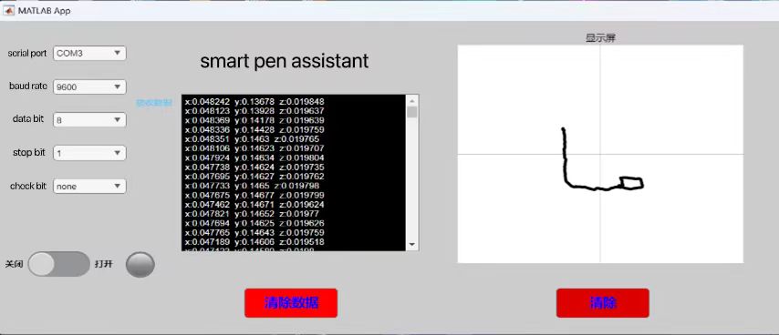
In the above figure, the left is the serial port information, the middle is the real-time three-axis magnetic induction intensity of the magnetic sensor array, and the right is the real-time handwriting display.

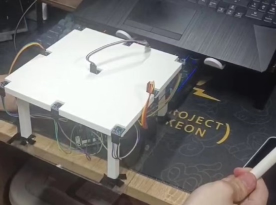
We designed and built a magnetic sensing array with a cylindrical magnet in a pen, and Figure 4 is a photograph of the real thing.

5. Conclusion

In this paper, the algorithm of magnetic sensor array positioning is discussed, the L-M algorithm is used to solve the equations, and the error causes of the magnetic sensor are discussed to improve the positioning accuracy. Finally, MATLAB was used to design an app to solve the uploaded data in real time and display handwriting. We have built the real thing, and the real thing has been tested to have good positioning accuracy, which can display handwriting in real time.

References

[1]. Thienen, Dieter Van et al. 2015. Smart Study: Pen and Paper-Based E-Learning.
[2]. Siddiqui, A. T., & Muntjir, M. 2017. An Approach to Smart Study using Pen and Paper Learning. International Journal of Emerging Technologies in Learning, 12(05), 117–27. https://doi.org/10.3991/ijet.v12i05.6798.
[3]. Tapia-Jaya, Ojeda-Zamalloa, et al. 2018. An Intelligent Pen to Assess Anxiety Levels Through Pressure Sensors and Fuzzy Logic. In: Ahram, T., Falcão, C. (eds) Advances in Human Factors in Wearable Technologies and Game Design. AHFE 2017. Advances in Intelligent Systems and Computing, vol 608. Springer, Cham. https://doi.org/10.1007/978-3-319-60639-2_7.
[4]. Wan'an Yang, Chao Hu, et al. 2010. A New Tracking System for Three Magnetic Objectives. IEEE Transactions on Magnetics, 46, 4023-29. https://doi.org/10.1109/TMAG.2010.2076823.
[5]. Gao Xiang, Shenggang Yan and Bin Li. 2017. A Novel Method of Localization for Moving Objects with an Alternating Magnetic Field. Sensors, 17, 923(1–12). https://doi.org/10.3390/s17040923.
[6]. Ding Haiyong, Bian Zhengfu. 2009. A Sub-pixel Registration Approach Based on Powell Algorithm. ACTA PHOTONICA SINICA, 38(12), 3322-27.
[7]. J. A. Nelder, R. Mead. 1965. A Simplex Method for Function Minimization. The Computer Journal, 7, 308-13.
[8]. Mattias Bjorkman, Kenneth Holmstrom. 1999. Global Optimization Using the DIRECT Algorithm in Matlab. Advanced Modeling and Optimization, 1(2), 17-29.
[9]. Waltraud Huyer, Arnold Neumaier. 1999. Global Optimization by Multilevel Coordinate Search. Journal of Global Optimization, 14, 331-55.
[10]. Lourakis. 2005. A Brief Description of the Levenberg-Marquardt Algorithm Implemened by levmar.
Cite this article
Ding,K. (2024). Design of an Intelligent Pen Based on Vector Magnetic Sensing. Applied and Computational Engineering,91,27-32.
Data availability
The datasets used and/or analyzed during the current study will be available from the authors upon reasonable request.
Disclaimer/Publisher's Note
The statements, opinions and data contained in all publications are solely those of the individual author(s) and contributor(s) and not of EWA Publishing and/or the editor(s). EWA Publishing and/or the editor(s) disclaim responsibility for any injury to people or property resulting from any ideas, methods, instructions or products referred to in the content.
About volume
Volume title: Proceedings of the 2nd International Conference on Functional Materials and Civil Engineering
© 2024 by the author(s). Licensee EWA Publishing, Oxford, UK. This article is an open access article distributed under the terms and
conditions of the Creative Commons Attribution (CC BY) license. Authors who
publish this series agree to the following terms:
1. Authors retain copyright and grant the series right of first publication with the work simultaneously licensed under a Creative Commons
Attribution License that allows others to share the work with an acknowledgment of the work's authorship and initial publication in this
series.
2. Authors are able to enter into separate, additional contractual arrangements for the non-exclusive distribution of the series's published
version of the work (e.g., post it to an institutional repository or publish it in a book), with an acknowledgment of its initial
publication in this series.
3. Authors are permitted and encouraged to post their work online (e.g., in institutional repositories or on their website) prior to and
during the submission process, as it can lead to productive exchanges, as well as earlier and greater citation of published work (See
Open access policy for details).