1. Introduction

To maintain the long goal of Early Childhood Longitudinal Studies(ECLS) program, the research is conducted primarily conducted to investigate and evaluate the effect of special education service brought to children’s later math performance. The children being studied come from diverse socioeconomic and racial/ethnic backgrounds. In addition to the reception of special education services regarded as the exposure variable in our study, children varied in other factors associated with demographic, academic, school composition, family context health and parent rating of child, which can all possibly influence their math test scores and may also impact their likelihood of receiving the special education services.

Thus, the situation remains consistent with the theory of causal inference pointing out the difficulty of calculating the accurate treatment effect in non-randomized experiments. The most widely used method to minimize the impact of confounding variables is propensity score analysis. Nowadays, lots of machine learning algorithms are proposed to predict the outcome values if the controlled groups were to be treated or the exposed group had not received treatment. By predicting the outcomes, the problem about randomization can be settled naturally. In our research, we applied Propensity Score Matching, Linear Regression, K-Nearest Neighbors, Bayesian Additive Regression Tree and Multi-Layers Perception to compute the average treatment effect(ATE). Besides, standard deviation(STD) of individual treatment effect is evaluated as well. By comparing the values of STD, more preferable methods stand out.

2. Literature Review

2.1. Traditional Causal Inference

Considering the potential causal relationship between observed features and past incidents, scientists proposed and developed the Rubin Causal Model to logically describe the causal inference, providing a meticulous and useful framework for experiments in causal inference. This model was applied in Holland and Rubin (1980) to analyze causal inference in retrospective, case-control studies used in medical research and in Holland and Rubin (1983) to analyze Lord's analysis of covariance" paradox[1]. In this model, we use the following notation: for each unit u in U, Y(u) is the response variable(the outcome). “S” indicates the exposure of the unit during the experiment. For all the units, they would either receive certain treatment or not, which is usually regarded as controlled. The two conditions are denoted as follows: \( S=t(treatment)/S=c(control) \) . Moreover, Y(u) are specified into \( {Y_{t}}(u) and {Y_{c}}(u) \) , representing the response value of all units in U exposed to 2 conditions respectively. The effect of cause is defined as \( {Y_{t}}(u) - {Y_{c}}(u) \) . Since \( {Y_{t}}(u) and {Y_{c}}(u) \) cannot be derived simultaneously for the same unit, which is called the Fundamental Problem of Causal Inference. To quantify the effect of cause statistically and solve the problem, the Rubin Causal Model puts forward several assumptions and utilizes the expectation. Considering ATE(Average Treatment Effect) as the variable indicating the quantified average effect of the cause, then we have the following equation:

\( ATE=E({Y_{t}}(u) -{Y_{c}}(u))=E({Y_{t}}(u))-E({Y_{c}}(u)) (1) \)

By this equation, we can derive the exact value of the effect by calculating the average of response values for the treated condition and the controlled condition separately and doing the subtraction. As is mentioned above, the model is based on several kinds of assumption:

Temporal Stability: It is assumed that the causal effect of the treatment on the outcome is stable over time and across subgroups within the population. The value of \( Y(u,c) \) does not depend on when the sequence "apply c to u then measure Y on u" occurs[1].

Causal Transience: The value of \( Y(u,t) \) is not influenced by the previous exposure of u to c.[1]

Unit Homogeneity: Scientists in the laboratory prepare two units \( {u_{1}},{u_{2}} \) conscientiously so that they appear identical in all relevant aspects to be convinced that \( Y({u_{1}},t)=Y({u_{2}},t) and Y({u_{1}},c)=Y({u_{2}},c) \) always hold.

Independence: This assumption can be interpreted as two equations:

\( \begin{cases}E({Y_{t}}(u))=E({Y_{t}}|S=t) \\ E({Y_{c}}(u))=E({Y_{c}}|S=c)\end{cases} (2) \)

Here, \( {E(Y_{t}}(u)) or E({Y_{c}}(u)) \) represents the average response value of all the units when exposed to t or c, while \( E({Y_{t}}|S=t) or E({Y_{c}}|S=c) \) means the average response value of part of the whole U with the exposure to t or c. If (2) holds, we have

\( T=E({Y_{t}}(u) -{Y_{c}}(u))=E({Y_{t}}(u))-E({Y_{c}}(u)) (3) \)

\( { T_{PF}}=E({Y_{t}}|S=t)-E({Y_{c}}|S=c) (4) \)

\( T={T_{PF }} (5) \)

By this formula, we can divide the original large sample into two parts (S=t/S=c) and observed the difference, recording the response value respectively.

Constant Effect: The effect of t on each unit u is regarded to be constant.

\( T={Y_{t}}(u)-{Y_{c}}(u)=constant, ∀u∈U (6) \)

If Unit Homogeneity holds, constant effect must be true, implying that Unit Homogeneity is a sufficient(stronger) condition for constant effect.

Randomized Controlled Trial&Exogenous Treatment Assignment: The units are randomly divided into two groups: one in the treatment group and one in the control group(S=t/S=c). The treatment outcome is the outcome that would occur if the individual received the treatment, while the control outcome is the outcome that would occur if the individual had not received the treatment. The assignment of treatments must be exogenous to the potential outcomes—meaning that it must not be systematically related to the potential outcomes.

No Unmeasured Confounders: Unmeasured confounders are ensured to be excluded, meaning that all factors that could affect both the treatment assignment and the outcome have been measured and controlled for, since it is critical to avoid biased estimates of causal effects.

Based on the Rubin Causal Model and our ideal hypothesis, we compute \( T=E({Y_{t}}(u) -{Y_{c}}(u))=E({Y_{t}}(u))-E({Y_{c}}(u)) \) . That is because the sample and the treatment are independent and will not influence each other, usually guaranteed by randomized experiment.

However, in most cases, without appropriate randomization, some experiments involve samples that will correlate with the treatment systematically, resulting in the inequality between \( E({Y_{t}}(u)) \) and \( E({Y_{t}}|S=t) \) and the equation of T will not hold. In such situation, we need to distinguish the disturbed one. So Propensity Score plays a key role by indicating the probability a unit receiving a particular treatment or intervention, given a set of observed characteristics or covariates.

\( Propensity Score≜P({S_{i}}=t|{U_{i}}) (7) \)

It can be calculated through Logistic Regression in several computer language such as R[2]. Moreover, Bayesian Network can also applied through structure learning to preclude non-causal relations[3].

2.2. Machine Learning in Causal Inference

With the development of computer science and statistics, when dealing with tremendous amounts of data, machine learning provides efficient and precise methodology for researchers to analyze the experimental data. In Causal Inference, numerous ML techniques have been developed and applied in various studies. Traditional method such as ordinary least squares(OLS) for linear regression has been widely used in many studies, but they were limited when encountering more complicated datasets. More new developed ML methods such as K nearest neighbors(KNN), Bidirectional and Auto-Regressive Transformers(BART), Optimal Discriminant Analysis(ODA), Neural Network(NN),etc[4,5,6,7].One research utilized BART model to compute a causal estimand called TEA to estimate the number of adverse health events prevented by large-scale air quality regulations via changes in exposure to multiple pollutants, which outperformed standard parametric approaches[4]. Neural Networks were applied to a new causal model by building a ML proxy predictor of the conditional average treatment effect, followed by the consequence showing the practical use of the method and its advantage to avoid making strong assumptions[5]. Moreover, the application of both regression-based algorithm and optimal discriminant analysis to estimate multi-valued treatment effects using data from an intervention including three study groups revealed that ODA is a robust alternative to conventional regression-based models for estimating effects in multivalued treatment studies due to its insensitivity to skewed data and use of accuracy measures applicable to all prognostic analyses[6]. Generally speaking, different data structures correspond to different causal methods[7]. In most cases, including the researches listed above, new ML models surpass traditional regression model.

3. Methodology

3.1. Overview of Our Experiment

The flowchart of our whole work:

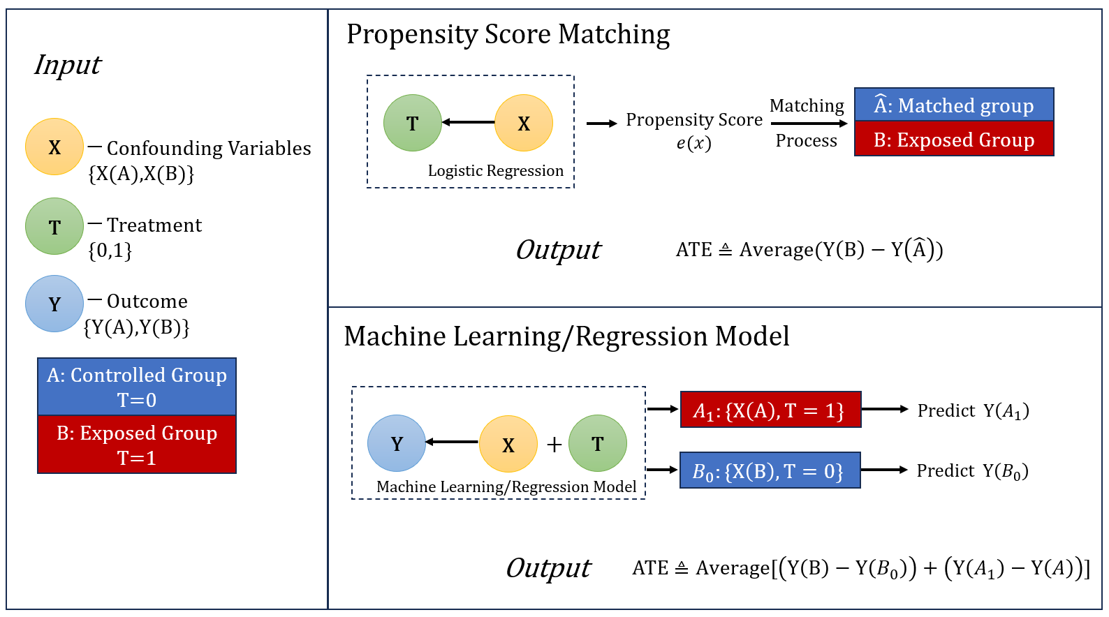
Figure 1. Flowchart of the Whole Research

3.2. Propensity Score Matching

As was mentioned before, in fact some experiments involve samples that will correlate with the treatment systematically, resulting in the inequality between \( E({Y_{t}}(u)) \) and \( E({Y_{t}}|S=t) \) . As a consequence, the difference between the outcomes of the controlled and the treatment groups does not merely shows the effect caused by the treatment but also those potentially contributed by the confounding variables.

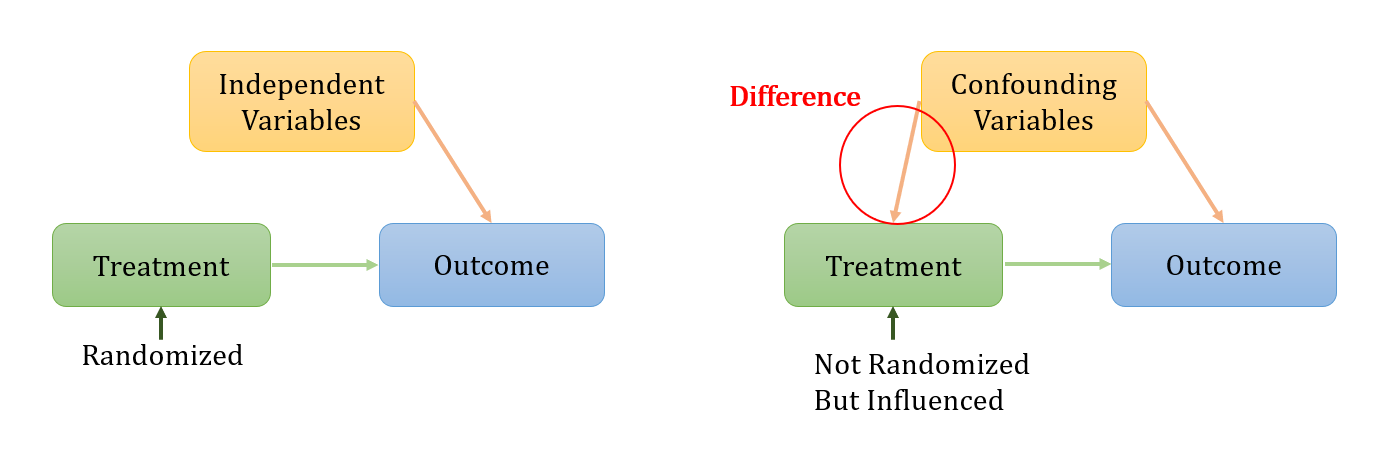
Figure 2. Relationships of Variables, Treatment and Outcome

Thus, Propensity Score Matching serves to construct an artificial control group by matching each treated unit with a non-treated unit of similar characteristics in order to reduce the error for estimating the treatment effect, which is a useful method in data analysis for estimating the impact of a program or event for which it is not ethically or logistically feasible to randomize. Let’s review the definition of propensity score:

\( Propensity Score≜P({S_{i}}=t|{U_{i}}) (8) \)

The score indicates the probability a unit receiving a particular treatment or intervention, given a set of observed characteristics or covariates. By knowing the definition, Propensity Score Analysis can be eventually divided into several steps. First, we need to collect data including all possible confounding variables that influence both the selection of treatment and the outcome variable. Then, having all the data, logistic regression model is commonly adopted as the propensity model to predict the propensity score equivalent to the probability of receiving the treatment given the confounders. By comparing the calculated propensity score, we manage to find a control record with the most similar propensity score for each example in the treatment group. Obtaining the match results, the quality of the matched records can be evaluated by comparing the similarity of the covariates. Finally, utilizing the new controlled group and the corresponding exposed group, the difference as well as the ATE can be computed.

3.3. Machine Learning Algorithms

3.3.1. Linear Regression: Ordinary Least Square

The most conventional method to analyze the correlations between the factors and the results is Linear Regression by Ordinary Least Square (OLS). The mentioned “Least Square” stands for the minimal square errors(SSE), which can be derived by adding the square differences of the observed and predicted values altogether.

Here we make the following assumptions:

the factor variables of all the trained objects:

\( X=(\begin{matrix}\begin{matrix}1 & {x_{11}} & {x_{12}} \\ 1 & {x_{21}} & {x_{22}} \\ \end{matrix} & \begin{matrix}⋯ & {x_{1n}} \\ ⋯ & {x_{2n}} \\ \end{matrix} \\ \begin{matrix}⋮ & ⋮ & ⋮ \\ 1 & {x_{m1}} & {x_{m2}} \\ \end{matrix} & \begin{matrix}⋱ & ⋮ \\ ⋯ & {x_{mn}} \\ \end{matrix} \\ \end{matrix}) \)

the observed values: \( Y={({y_{1}},{y_{2}},⋯,{y_{m}})^{T}} \) the predicted value: \( \hat{Y}={({\hat{y}_{1}},{\hat{y}_{2}},⋯,{\hat{y}_{m}})^{T}} \)

Since we assume the relation between the influential factors and the results can be expressed linearly, there exist \( β={({{β_{0}},β_{1}},{β_{2}},⋯,{β_{n}})^{T}} \) such that \( \hat{Y}=Xβ \)

By the definition of square errors, we have

\( SSE=\sum _{i=1}^{m}{({\hat{y}_{i}}-{y_{i}})^{2}}={(\hat{Y}-Y)^{T}}(\hat{Y}-Y)={(Xβ-Y)^{T}}(Xβ-Y) (9) \)

The aim is to find the optimal \( {β^{*}} \) to minimize SSE. Therefore, by the necessary optimal condition, it is required that \( {∇_{SSE}}({β^{*}})=0 \) i.e. \( 2{X^{T}}(X{β^{*}}-Y)=0 \)

Finally, we can derive the optimal coefficients for the linear regression:

\( {β^{*}}={{({X^{T}}X)^{-1}}X^{T}}Y (10) \)

More specifically, if only one factor is researched, we have \( X={(\begin{matrix}{x_{1}} \\ 1 \\ \end{matrix} \begin{matrix}{x_{2}} \\ 1 \\ \end{matrix} \begin{matrix}⋯ \\ ⋯ \\ \end{matrix} \begin{matrix}{x_{m}} \\ 1 \\ \end{matrix})^{T}},β={({{β_{0}},β_{1}})^{T}} \)

\( SSE=\sum _{i=1}^{m}{({\hat{y}_{i}}-{y_{i}})^{2}}=\sum _{i=1}^{m}{({β_{1}}{x_{i}}+{β_{0}}-{y_{i}})^{2}} (11) \)

By the necessary optimal condition, we have

\( \begin{cases}{∇_{SSE}}(β_{1}^{*})=2\sum _{i=1}^{m}{x_{i}}({β_{1}}{x_{i}}+{β_{0}}-{y_{i}})=0 (12) \\ {∇_{SSE}}(β_{0}^{*})=2\sum _{i=1}^{m}{(β_{1}}{x_{i}}+{β_{0}}-{y_{i}})=0 (13)\end{cases} \)

Solving the equations, the coefficients can be precisely calculated as:

\( \begin{cases}β_{1}^{*}=\frac{\sum _{i=1}^{m}({x_{i}}-\bar{x})({y_{i}}-\bar{y})}{\sum _{i=1}^{m}{({x_{i}}-\bar{x})^{2}}} (14) \\ β_{0}^{*}=\bar{y}-β_{1}^{*}\bar{x} (15)\end{cases} \)

3.3.2. KNN Algorithm

Different from traditional methods, machine learning excels by its robust adaptability for various datasets. K-Nearest Neighbor Algorithm(KNN) is a widely used machine learning technique. After calculating the distance between input data and all the training sample points, the algorithm select K(the number of the selected points) nearest neighboring samples. For classification, the most common labels among the chosen neighbors is regarded as the predicted label of the input data. For regression, we assign the (weighted) average of the sample values of the neighbors as the predicted value of the input data. Obviously, the performance of the algorithm depends on parameter “K” and the distance metric[8].

Usually, the distance metric is determined among the following:

Euclidean distance( \( {‖x‖_{2}} \) ):

\( d(x,y)=\sqrt[]{\sum {({y_{i}}-{x_{i}})^{2}}} (16) \)

Manhattan distance( \( {‖x‖_{1}} \) ):

\( d(x,y)=\sum |{y_{i}}-{x_{i}}| (17) \)

Minkowski distance( \( {‖x‖_{p}} \) ):

\( d(x,y)={(\sum {({y_{i}}-{x_{i}})^{p}})^{\frac{1}{p}}} (18) \)

3.3.3. Bayesian Additive Regression Tree

Combining the idea of regression and tree-based model, Bayesian Additive Regression Tree(BART) algorithm utilize sum of trees to approximate an unknown function \( f \) . Suggesting there is an unknown function \( f \) for predicting \( y \) based on the input \( x \) :

\( y=f(x)+ε, ε~N(0,{σ^{2}}) (19) \)

BART uses sums of trees \( \sum {g_{j}}(x) \) where \( {g_{j}}(x) \) denotes a regression tree to approximate the unknown function \( f \) :

\( f(x)≈h(x)=\sum _{j=1}^{m}{g_{j}}(x) (20) \)

\( ⟹y=h(x)+ ε, ε~N(0,{σ^{2}}) (21) \)

Let T denote a binary tree and assume the tree has b terminal nodes, then \( M=({μ_{1}},{μ_{2}},⋯,{μ_{b}}) \) represents the parameter values corresponding to each of the terminal nodes. So, for a binary tree, each input value x is associated with a single terminal node of T and is then assigned the \( {μ_{i}} \) value corresponding to this node. Given the input x and the tree T with a set of parameters M, the regression tree can be denoted as \( g(x;T,M) \) .

Based on this notation, the sum-of trees model can be mathematically written as:

\( y=\sum _{j=1}^{m}g(x;{T_{j}},{M_{j}})+ ε, ε~N(0,{σ^{2}}) (22) \)

For each binary regression tree \( {T_{j}} \) , a set of parameters \( {M_{j}}=({μ_{1j}},{μ_{2j}},⋯,{μ_{bj}}) \) is associated with the tree’s terminal nodes.

The sum-of-trees model manage to incorporate both main effects and interaction effects. Large number of trees endows BART algorithm with robust predictive capabilities. For a fixed number of trees as m, \( ({T_{1}},{M_{1}}),⋯,({T_{m}},{M_{m}}),σ \) finally specify the sum-of-trees model, which is completed by imposing a prior over all the parameters aiming to limit the scale of individual tree preventing their effects from being exceedingly influential.

Firstly, it is assumed that the tree components \( ({T_{j}},{M_{j}}) \) are independent of each other as well as \( σ \) and the terminal node parameters of every tree are independent.

Then we have the following equations:

\( p(({T_{1}},{M_{1}}),⋯,({T_{j}},{M_{j}}),σ)=p(σ)\ \ \ (23) \)

\( =p(σ) (24) \)

\( p({M_{j}}{T_{j}})= (25) \)

According to equation (24) and (25),1. the original specification problem is converted into the specification of \( p({T_{j}}), p({μ_{ij}}{T_{j}}) and p(σ). \) So the prior is separated into three parts: the \( {T_{j}} \) prior, the \( {μ_{ij}}|{T_{j}} \) prior, and the \( σ \) prior.

1) The \( {T_{j}} \) prior

The distribution on the splitting variable assignments and the distribution on the splitting rule assignment is the uniform prior on each binary tree distribution. In addition, the probability that a node at depth \( d=(0,1,2,⋯) \) is nonterminal require further specification. The specification is given by: \( \frac{α}{{(1+d)^{β}}}, α∈(0,1) and β∈[0,∞) \) . To keep individual tree components small, usually we adopt \( α=0.95 and β=2 \) .

2) The \( {μ_{ij}}|{T_{j}} \) prior

The output data y will be rescaled ranging from \( {y_{min}}=-0.5 to {y_{max}}=0.5 \) .

Then the prior is:

\( {μ_{ij}}~N(0,σ_{μ}^{2}), {σ_{μ}}=\frac{0.5}{k\sqrt[]{m}} (26) \)

The prior exerts the effort to shrink the parameter \( {μ_{ij}} \) toward zero. When k or m increases, the shrinkage to the \( {μ_{ij}} \) accelerates, making the prior tighter.

3) The \( σ \) prior

The prior exploit inverse chi-square distribution:

\( {σ^{2}}~\frac{υλ}{χ_{υ}^{2}} (27) \)

where \( υ \) stands for the degree of freedom and \( λ \) is the scale.

We calibrate the prior for the degree of freedom \( υ \) and scale \( λ \) for this purpose using a rough data-based overestimate \( \hat{σ} \) of \( σ \) . Usually, there are two natural choices: naïve specification (the sample standard deviation of sample y) and the linear model specification (the residual standard deviation from a least squares linear regression of y on the original X). Then a value of \( υ \) is picked between 3 and 10 to derive an appropriate shape and a value of \( λ \) is chosen such that the \( q \) th quantile of the prior on \( σ \) is located at \( \hat{σ} \) . The value of \( q \) is always considered such as 0.75,0.90 or 0.99 to center the distribution below \( \hat{σ} \) .

For automatic use, Chipman et al. [9] recommend the default setting \( (ν,q)=(3,0.90) \) .

For the fixed tree number \( m \) , a fast and robust option is to set \( m \) as 200.

Given the observed data y of the sample value x, the Bayesian setup induces a posterior distribution:

\( p(({T_{1}},{M_{1}}),⋯,({T_{j}},{M_{j}}),σ| y) (28) \)

Through approaches such as a backfitting MCMC algorithm proposed by Chipman et al. [9] and Particle Gibbs proposed by Lakshminarayanan et al. [10], the parameters can be specified.

As a consequence, the BART model can successfully output a posterior mean estimate of \( f(x)=E(y | x) \) .

Table 1. Iteration of BART Algorithm

3.3.4. Neural Network: Multi-Layer Perception

Among machine learning techniques, Neural Network is a popular method. Its archetypical model Multi-layer Perceptron is a supervised learning algorithm that learns a function \( f: {R^{m}}⟶{R^{o}} \) by training on a dataset where \( m \) is the number of dimensions for input and \( o \) is the number of dimensions for output. Given a set of features \( X={x_{1}},{x_{2}},⋯,{x_{m}} \) and a target y, it can learn a non-linear function approximator for either classification or regression. The model consists of multiple non-linear layers usually called the hidden layers.

Without loss of generality, we can assume now we have input data \( X={x_{1}},{x_{2}},⋯,{x_{m}} \) and the hidden layer \( H={h_{1}},{h_{2}},⋯,{h_{o}} \) . The model serves to compute the target value y.

For each element \( {x_{i}} \) , it has a set of weight values \( \lbrace {w_{i1}},{w_{i2}},⋯,{w_{io}}\rbrace \) corresponding to the calculation of the elements in the hidden layer:

where f is a function which can be either linear or non-linear(more often).

Three types of commonly adopted funcitons:

1) relu:

\( y=max(0,x) (30) \)

2) tanh: \( \)

\( y=\frac{{e^{x}}-{e^{-x}}}{{e^{x}}+{e^{-x}}} (31) \)

3) sigmoid:

\( y=\frac{1}{1+{e^{-x}}} (32) \)

Then for the hidden layer \( H \) , each element has a set of weight values for the next layer.

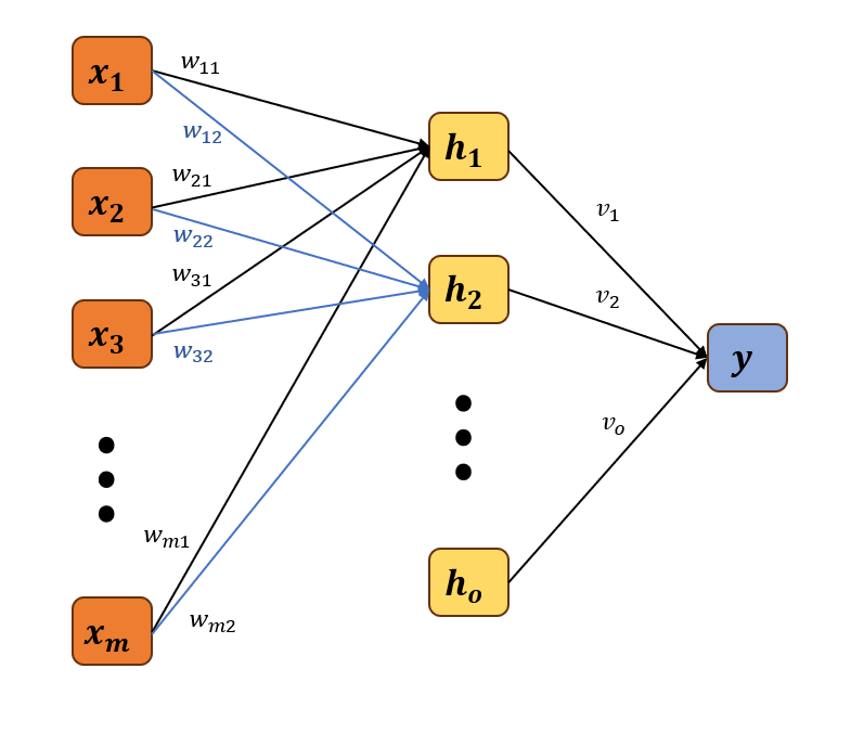
Figure 3. Working Mechanism of MLP

If the hidden layer is the last layer before the output data as the graph shows, then we can calculate the target value y:

Since there are several numerous parameters involved in the computing process, they need to be specified. They are specified to obtain the minimized error for the training datasets.

If we denote the predicted target values for the training data as \( \hat{y}=({\hat{y}_{1}},{\hat{y}_{2}},⋯,{\hat{y}_{n}}) \) where n is the sample size and consider \( y=({y_{1}},{y_{2}},⋯,{y_{n}}) \) as the observed data.

Then the error can be described as:

\( ‖y-\hat{y}‖_{2}^{2}=\sum _{i=1}^{n}{({y_{i}}-{\hat{y}_{i}})^{2}} (34) \)

Since the predicted value \( \hat{y} \) was determined by parameter \( {({w_{ij}})_{m×o}}, b, {v_{i}} \) and \( s \) , we can also denote the error as a loss function: \( L(ϕ(x;w,b,v,s),y) \) . Then to derive the most satisfying parameters, we need to solve the following optimization problem:

\( \underset{w,b,v,s}{min}{L(ϕ(x;w,b,v,s),y)} (35) \)

Usually for optimization, there are approaches for us to adopt to compute the solutions, such as Stochastic Gradient Descent(SGD), momentum method, Nesterov Accelerated Method and AdaGrad/RMSProp/AdaDelta/Adam Algorithms.

4. Experiment and Result

4.1. Data Description

In our experiment, the data originally come from the Early Childhood Longitudinal Studies (ECLS) program, Kindergarten Class of 1998-1999 (ECLS-K). The dataset contains a wide range of family, school, community, and individual factors related to children's development, early learning, and performance in school. To be more detailed about our evaluation about the causal inference, the covariates consist of factors related to demographic, academic, school composition, family context, health and parent rating of child. The treatment here is indicated by the exposure variable “Special Education Services” which is denoted as F5SPECS. For the purpose of the ECLS-K, children with disabilities are those who meet the federal eligibility requirements for participation in special education programs or services. All children with disabilities are expected to have an Individualized Education Plan (IEP), an Individualized Family Service Plan (IFSP), or a 504 Plan on file with the school district as it is a required component of the eligibility process.

After data pre-processing, the whole datasets consisted of 7362 cases, 429 of which received special education services. Whether a child was regarded as a recipient of special education services depended on their special education status gathered from school administrative records from the spring of 2002[2]. According to the past analysis in an issue brief by IES describing Demographic and School Characteristics of Students Receiving Special Education in the Elementary Grades[11], for the cohort of students beginning kindergarten in 1998, specific learning disabilities and speech or language impairments were the most prevalent primary disabilities over the grades studied.Higher percentages of boys than girls and of poor students than non-poor students received special education. In each grade studied, public schools reported higher percentages of students receiving special education than did private schools.

Meanwhile, the ECLS-K Revised IRT scaled math achievement test score ranging from 50.9 to 170.7 is considered the outcome variable.

4.2. Result and Experiment of Causal Inference

In the coding process, we mainly chose python to run the models through different models to calculate the average treatment effect and the standard deviation of individual treatment effect. By comparing the the standard deviation of individual treatment effect, we can assess the performance of all the applied methods. The computing process can be categorized into two parts composed of different steps to solve the fundamental problem of calculate treatment effect:

1) In the method of Propensity Score Matching, we first adopt logistic regression based on the covariates and the exposure variable to compute the probability of each individual receiving the treatment with their covariates information. By matching the exposed individual(n=429) with the controlled one having the closest score to the exposed one and then subtracting the controlled score from the exposed score, we can derive individual treatment effect and compute ATE and the standard deviation of ITE(n=429).

2) In the machine learning part, by applying the packages that are already created for logistics regression, OLS, KNN, BART, MLP on the whole datasets, we trained models predicting the outcomes based on the covariates and the exposure variables. Then we reversed the exposure variables(changing 0 to 1, changing 1 to 0) and evaluate new outcomes. Eventually, we obtain the response variables of the whole datasets(n=7362) under both circumstances. Subtracting the controlled score from the exposed score, we derive the individual treatment effect and compute ATE and the standard deviation(STD) of ITE(n=7362).

Table 2. ATE & Standard deviation of Individual Treatment Effect computed by Listed Algorithms

Surprisingly, the average treatment effects of Special Education Services calculated turn out to be all minus. Besides, the standard deviation revealed that KNN, OLS and BART are more stable with better performances in calculating ATE. Whereas, MLP and PSM brought higher STD values indicating the fluctuation of the individual treatment effect among the datasets.

4.3. Factor Analysis

It may seem surprising that the treatment effect evaluated turned out to be minus. Since the datasets containing 7363 sets of data only have 429 test takers experiencing special education services. So the minority of the exposed individuals suggesting some hidden selection bias serves as a possible reason explaining why the average treatment effects calculated by all methods are minus.

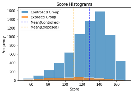
Figure 4. Histograms of Math Scores of Controlled and Exposed Groups

Table 3. Mean and Standard Deviation of Math Scores of Controlled and Exposed Groups

According to the histograms of the controlled and the exposed group, we can easily conclude that scores of exposed group are symmetrically distributed. Comparatively, the controlled scores are skewed toward higher scores. Consequently, the mean score of controlled group is originally higher than the one of the exposed score. Thus, we can probably speculate that the exposed group receiving special educational service have potential disadvantage inherently such as intelligence disabilities or psychological problems in terms of math performance. Meanwhile, when the machine learning algorithms begins to learn the datasets, the higher scores are often appeared without the special treatment. Vice Versa, the special treatment is always accompanied by lower math scores, leading the trained model to predict higher/lower scores when treatment variable turns into 0/1, which finally caused the difference to be minus. What factors actually cause the outcomes to be different? Here we adopt the traditional regression method OLS to compute the results showing the influencing coefficient of all the factors. Compare with other machine learning algorithms, OLS excels in its ability to quantify the relationships of the factors and outcomes.

Table 4. Contributing Parameters of Variables to Math Scores(OLS)

The table illustrates the highly influencing factors with high absolute values of the coefficients include whether the child go to public school, the child’s genders, whether the child receive special education services and whether the child is a first-time kindergartener.

Except the factor of special education services that is negatively related to the math scores, the other three factors are all positively related to the output variables and the identity of first-time kindergartner contributes the most.

Having found the outstanding influential factors and their relations with the final outcomes, let’s check those factors ’distribution in the controlled and exposed group respectively.

Since all the influential factors are recorded by binary response, here we calculated the frequency of two categories of the answer \( \lbrace 0,1\rbrace \) in the controlled and exposed group in order to distinguish the differences.

For the factor of special education services causing decline of the score, apparently the exposed group are 100% receiving the services. The most influential factor which is the identity of first-time kindergartner has higher frequency among the controlled group than the exposed group, which also help explain why the controlled group performed better in the math test. Whereas, the other positively-related factors consisting of gender and public school turned out to be in favor of the exposed groups’ scores. Nevertheless, with the largest influential parameter of first-time kindergartner and isolation from treatment services, the controlled group still outperformed the exposed one.

To dig and explore the more distinguished characteristics of the factors, Principle Components Analysis(PCA) is also adopted here on the whole datasets outputting continuous component variables. Applying Principle Components Analysis(PCA) on all the characteristics of individual including the covariates and the exposure variable, we found out that 6 principle components accounted for 95% of all the components.

Table 6. Constituting Parameters of Variables in PC1~PC6(PCA)

The parameters of the principal components in the table shows that among all the features of the individuals, the group of factors about family context is embedded in the 6 components to the greatest extent followed by health, school composition and academic progressively.

All those components mainly indicates the variances of individuals.

Table 7. Contributing Parameters of PC1~PC6 to Math Scores(OLS)

Just like the way we had selected primary influencing factors before PCA, we utilized OLS for regression analysis and chose PC1,PC2 and PC6 with high absolute values of coefficients as our main investigated variables. The coefficient table reveals that PC5 and PC6 play significant role in enhancing the math scores while PC1 affects negatively.

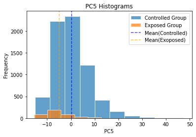
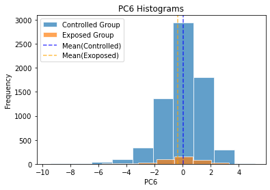
By comparing the distribution and the mean value of each group, we found that the controlled group has relatively higher values of PC5 and PC6 and lower value of PC1. The variations of all these three components contribute to greater outputs of the controlled group. The results derived from the projected data after PCA show more consistent and less antagonistic impact of the factors, which help verify the effectiveness of PCA adoption on our datasets.

5. Conclusion

First, in terms of the standard deviation of the ITE, all the machine learning algorithms with comparatively low STD outperformed the traditional propensity score matching. Among those machine learning algorithms, KNN, BART and OLS excelled, offering much more stable calculations.

Moreover, the values of ATE computed through all the methods turned out to be below zero. The results of factor analysis revealed that kids’ math scores has intensively positive relationships with the identity of first-time kindergartners and Kindergarten Math Scores while strongly impaired by the Number of Siblings and Non-parental Pre-K Child Care. The controlled group boasted more first-time kindergartner and higher Kindergarten Math Scores with smaller Number of Siblings and less Non-parental Pre-K Child Care, reasonably causing the greater performance in the math test scores. The machine learning algorithms learned that higher scores often appeared without the special treatment. Thus, special treatment effect led the trained model to predict lower scores, which finally caused the difference to be negative.

References

[1]. Holland, P. W. (1986). Statistics and Causal Inference. Journal of the American Statistical Association, 81(396), 945–960. https://doi.org/10.1080/01621459.1986.10478354
[2]. Keller, B., & Tipton, E. (2016). Propensity score analysis in R: A software review. Journal of Educational and Behavioral Statistics, 41(3), 326-348. https://doi.org/10.3102/1076998616631744
[3]. Sieswerda, M., Xie, S., et al. (2023). Identifying confounders using bayesian networks and estimating treatment effect in prostate cancer with observational data. JCO Clinical Cancer Informatics, 7, e2200080. https://doi.org/10.1200/CCI.22.00080
[4]. Nethery, R. C., Mealli, F., Sacks, J. D., & Dominici, F. (2019). Causal inference and machine learning approaches for evaluation of the health impacts of large-scale air quality regulations. arXiv preprint arXiv:1909.09611. https://doi.org/10.48550/arXiv.1909.09611
[5]. Chernozhukov, V., Demirer, M., Duflo, E., & Fernandez-Val, I. (2018). Generic machine learning inference on heterogeneous treatment effects in randomized experiments, with an application to immunization in India (No. w24678). National Bureau of Economic Research. https://www.nber.org/papers/w24678
[6]. Linden, A., & Yarnold, P. R. (2016). Combining machine learning and propensity score weighting to estimate causal effects in multivalued treatments. Journal of Evaluation in Clinical Practice, 22(6), 875-885. https://doi.org/10.1111/jep.12610
[7]. Parikh, H., Varjao, C., Xu, L., & Tchetgen, E. T. (2022, June). Validating causal inference methods. In International conference on machine learning (pp. 17346-17358). PMLR.
[8]. What is the K-nearest neighbors algorithm?. IBM. (2021, October 4). https://www.ibm.com/topics/knn
[9]. Chipman, H. A., George, E. I., & McCulloch, R. E. (2010). BART: Bayesian additive regression trees. https://doi.org/10.1214/09-AOAS285
[10]. Lakshminarayanan, B., Roy, D., & Teh, Y. W. (2015, February). Particle Gibbs for Bayesian additive regression trees. In Artificial Intelligence and Statistics (pp. 553-561). PMLR.
[11]. U.S. Department of Education. (2007a, July). Demographic and School Characteristics of Students Receiving Special Education in the Elementary Grades. AIR. https://www.air.org/project/early-childhood-longitudinal-studies-ecls
Cite this article
Huang,L. (2024). Machine learning and propensity score matching for evaluating the effect of special education services on children’s later math performances. Applied and Computational Engineering,88,218-233.
Data availability
The datasets used and/or analyzed during the current study will be available from the authors upon reasonable request.
Disclaimer/Publisher's Note
The statements, opinions and data contained in all publications are solely those of the individual author(s) and contributor(s) and not of EWA Publishing and/or the editor(s). EWA Publishing and/or the editor(s) disclaim responsibility for any injury to people or property resulting from any ideas, methods, instructions or products referred to in the content.
About volume
Volume title: Proceedings of the 6th International Conference on Computing and Data Science
© 2024 by the author(s). Licensee EWA Publishing, Oxford, UK. This article is an open access article distributed under the terms and
conditions of the Creative Commons Attribution (CC BY) license. Authors who
publish this series agree to the following terms:
1. Authors retain copyright and grant the series right of first publication with the work simultaneously licensed under a Creative Commons
Attribution License that allows others to share the work with an acknowledgment of the work's authorship and initial publication in this
series.
2. Authors are able to enter into separate, additional contractual arrangements for the non-exclusive distribution of the series's published
version of the work (e.g., post it to an institutional repository or publish it in a book), with an acknowledgment of its initial
publication in this series.
3. Authors are permitted and encouraged to post their work online (e.g., in institutional repositories or on their website) prior to and
during the submission process, as it can lead to productive exchanges, as well as earlier and greater citation of published work (See
Open access policy for details).