1. Introduction

Time series forecasting involves predicting future trends, patterns, or values by analyzing historical data and is widely used across many fields. In the financial and economic sectors, it can predict market trends and macroeconomic indicators [1]. In meteorology, it forecasts weather and climate change [2]. In public health, it projects disease trends [3]. Time series forecasting provides accurate insights into future developments, which are invaluable for resource optimization, risk management, and decision support. This method holds significant social relevance and research value.

The mainstream methods of time series forecasting can primarily be classified into traditional methods and machine learning-based methods. The traditional time series analysis methods typically complete the forecasting by analyzing the mathematical or statistical properties of the data. George Box et al. [4] incorporated autocorrelation and partial autocorrelation functions into the differential autoregressive moving average model. Through model identification, parameter estimation, and diagnostic checking of the time series data modeling, they effectively analyzed and forecasted the aviation data set, achieving a root mean square error of 0.037. Robert F. Engle [5] utilized autoregressive conditional heteroskedasticity for time series forecasting, creating a time-dependent variance series. This model considers the time-varying nature of volatility and accurately captures the dynamics among high and low volatility periods, successfully predicting the inflation rate in the U.K. Charles C. Holt [6] extended the simple exponential smoothing method to address the trend component of the data, enhancing the prediction accuracy for time series with trends. Sean J. Taylor et al. [7] introduced a decomposable time series model that accounts for trend, periodicity, and specific events, efficiently forecasting time series with seasonal characteristics and event impacts. Although traditional methods can yield good results under certain conditions, they heavily rely on human-designed parameter adjustments when building the model. Consequently, it is often challenging to fully extract the characteristics of the time series, limiting the prediction accuracy, especially for nonlinear and non-smooth time series.

In recent years, with the development of artificial intelligence and improvements in graphics card processing, machine learning methods have been widely used in the field of time series forecasting. Mehrnaz Ahmadi and Mehdi Khashei [8] addressed deterministic and uncertain patterns in data by separately combining a support vector machine with a fuzzy support vector machine, and finally used another support vector machine to integrate the different models. Xueheng Qiu [9] selected linear combinations of features by applying a least squares classifier at each node of the decision tree, allowing the random forest model to consider multiple linear combinations of features simultaneously. This approach captures the complex structure of data and has demonstrated strong robustness in forecasting electricity load demand in the Australian energy market. Mst Noorunnahar et al. [10] utilized XGBoost for time series forecasting by using an optimized gradient boosting algorithm and aggregating outputs from multiple decision trees. This method predicted the annual rice production in Bangladesh with an average absolute percentage error of 5.38%, outperforming the ARIMA model’s 7.23%. Beyond the earlier mentioned machine learning techniques, neural network-based deep learning models are increasingly being utilized. Samit Bhanja and Abhishek Das [11] improved recurrent neural networks by introducing multiple hidden layers, which enabled the model to efficiently learn complex sequential dependencies and nonlinear relationships, thus improving prediction of future data points. Ryan Solgi et al. [12] employed a long short-term memory network to process time series data, effectively capturing and utilizing long-term dependencies in historical data to accurately predict future changes in groundwater levels. Haiping Lin et al. [13] used a gated recurrent unit (GRU) network model to process sequence data. Through a multilayer network structure and variational mode decomposition technique, the model enhanced learning capabilities and prediction accuracy for long-term sequence data, successfully predicting groundwater data changes. Machine learning methods can flexibly handle nonlinear relationships and are suitable for many types of time series data. However, traditional machine learning algorithms are highly dependent on manually selected features and often require complex data preprocessing. In contrast, neural network-based methods facilitate end-to-end automatic feature extraction but require significant computational resources for training, which is costly and may lead to issues such as overfitting.

To address the issues mentioned, this paper proposes a time series prediction method based on feature fusion and XGBoost. Initially, the data are preprocessed, and feature extraction is performed using algorithms such as K-Means to enhance the feature set. Subsequently, XGBoost is employed for predicting the time series. The XGBoost algorithm requires fewer computational resources and is less complex to implement compared to methods like LSTM. Consequently, our method can efficiently and effectively accomplish the task of time series prediction.

2. Methodology

2.1. K-means clustering algorithm

The K-means algorithm is an unsupervised algorithm for cluster analysis, developed by Hugo Steinhaus [14], Stuart Lloyd [15], and Robert C. Jancey [16], among other researchers in various fields. The method is simple, efficient, and widely used across numerous domains.

K-means excels at extracting unnoticed behaviors and patterns from data without any prior knowledge, clustering time series data into several groups with similar trends and patterns. Additionally, the K-means clustering algorithm is highly efficient in handling large-scale datasets, making it suitable for analyzing and clustering substantial amounts of data. Therefore, we employ this algorithm for the preliminary feature extraction of our time series dataset. The main process of this algorithm is outlined as follows:

Initially, k points are selected as the initial centers: m1(1), m2(1), m3(1) ..., mk(1) . The algorithm then follows an iterative loop process to optimize the centroid locations:

(1) Assignment: Traverse each data point xp, and assign it to the centroid with the least squares Euclidean distance, mathematically expressed as follows:

\( S_{i}^{(t)​}=\{x_{p}​:∥x_{p}​ - m_{i}^{(t)}∥^{2}≤∥x_{p}​ - m_{j}^{(t)}​∥^{2},∀j,1≤j≤k\}\ \ \ (1) \)

In equation (1). \( S_{i}^{(t)​} \) denotes the set of 𝑖-th cluster at the 𝑡-th iteration.

(2) Update: After each assignment, the algorithm updates the centroid of each cluster with the mean value of all points in the current cluster as follows:

\( m_{i}^{(t+1)}=\frac{1}{|S_{i}^{(t)}|}\sum _{x_{j}∈S_{i}^{(t)}}^{} x_{j}\ \ \ (2) \)

In equation (2). \( m_i^{(t+1)} \) denotes the new centroid of the 𝑖-th cluster at the (t+1)-th iteration.

The process is repeated iteratively until one of the following termination conditions is met: (a) a preset number of iterations is reached, or (b) the change in all cluster centers over two consecutive iterations is less than the tolerance.

Upon termination, the algorithm outputs the final centroids of each cluster and the data points within the cluster.

2.2. XGBoost

XGBoost (eXtreme Gradient Boosting), proposed by Tianqi Chen et al. in 2014 [17], is an efficient and flexible gradient boosting framework. It optimizes the objective function by iteratively constructing decision trees and is applicable to common supervised learning tasks such as classification, regression, and ranking.

Our experimental dataset exhibits strong time series characteristics and contains complex nonlinear patterns. XGBoost can learn these nonlinear relationships by constructing multiple gradient boosting decision trees, making it more effective than traditional models such as ARIMA, which often struggle with complex nonlinear patterns. The integration of multiple decision trees enhances the resilience of XGBoost against outliers and noise, enabling the model to effectively mitigate the impact of unexpected events during prediction. Additionally, XGBoost effectively reduces the risk of overfitting through the use of common regularization techniques, such as L1 and L2 regularization. These attributes make XGBoost highly suitable for completing time series predictions efficiently, which aligns well with the research objectives of this paper. The main workflow of the algorithm is as follows:

A constant value, \[ \hat{f}​^{(0)}(x) \] is initially used to initialize the model. This constant is calculated by minimizing the loss function:

\( \hat{f}​^{(0)}(x)=argmin_{θ}​∑_{i=1}^{N}​L(y_{i}​,θ)\ \ \ (3) \)

In Eq. (3), θ is the parameter of the model, 𝐿(𝑦𝑖 ,𝜃) is the loss function, and 𝑦𝑖 is the true label of the training data.

Then, the algorithm iteratively adds weak learners. For each iteration 𝑚, from 1 to 𝑀, the following steps are performed:

(1) Gradient and curvature calculation: Calculate the gradient and second-order derivatives for each data point under the current model to evaluate the curvature of the loss function. This allows the model predictions to be adjusted in the direction that reduces the overall loss, ensuring stable and efficient model updates:

\( \hat{g}_{m}(x_{i})=[\frac{∂L(y_{i}​,f(x_{i}))}{∂f(x_{i})}​]_{f(x)=\hat{f}_{(m - 1)}(x)}​ \ \ \ (4) \)

\( \hat{h}_{m}(x_{i})=[\frac{∂^{2}L(y_{i}​,f(x_{i}))}{∂f(x_{i})^{2}}​]_{f(x)=\hat{f}_{(m - 1)}(x) }​\ \ \ (5) \)

In equation (4), \( x_i \) denotes the ith data point, and \( {\hat{g}}_m(x_i) \) represents the gradient, which is the first-order derivative of the loss function with respect to the current model prediction. It indicates the growth rate of the loss function at each data point. In Eq. (5), \( {\hat{h}}_m(x_i) \) represents the second-order derivative of the loss function relative to the current model prediction, describing the rate of change of the gradient.

(2) In the gradient boosting approach, our goal is to reduce the overall model prediction error by fitting a new weak learner. To this end, the new weak learner is fitted with the objective of minimizing the ratio of the negative value of the gradient to the second-order derivative. This method utilizes the gradient information to guide the learning process, effectively allowing the weak learner to optimize directly for error reduction. The specific mathematical expression is described as follows:

\( \hat{ϕ}_{m}​=argmin_{ϕ∈Φ}​∑_{i=1}^{N}​\frac{1}{2}​\hat{h}_{m}(x_{i})[ϕ(x_{i}​) - \frac{\hat{g}_{m}(x_{i})}{\hat{h}_{m}(x_{i})}]^{2}\ \ \ (6) \)

In equation (6). \( {\hat{\phi}}_m​ \) represents the weak learner.

(3) Update model parameters: the newly learned model \( {\hat{f}}_m(x) \) is added to the existing model by multiplying by the learning rate 𝛼. This step is cumulative, meaning that the output of each iteration builds upon the previous one:

\( \hat{f}_{m}(x)=α\hat{ϕ}_{m}​(x)\ \ \ (7) \)

\( \hat{f}_{(m)}(x)=\hat{f}_{(m - 1)}(x)+\hat{f}_{m}(x)\ \ \ (8) \)

Ultimately, the XGBoost output is an accumulation of the models learned from all iterations:

\( \hat{f}(x)=∑_{m=0}^{M}​\hat{f}​_{m}​(x)\ \ \ (9) \)

2.3. LSTM (Long Short-Term Memory network) and GRU

LSTM (Long Short-Term Memory networks) and GRU (Gated Recurrent Unit networks) are two types of recurrent neural networks that facilitate the analysis and prediction of time series through a multilayer network structure. LSTM was introduced by Hochreiter S. and Schmidhuber J. in 1997 [18], while GRU was developed by Cho K. et al. in 2014 [19].

Both LSTM and GRU are designed to effectively capture long-term dependencies in time series data by regulating the flow of information through the structure of "gates," which selectively remember and forget information. Unlike traditional and other machine learning methods that require manual feature engineering, LSTM and GRU can automatically extract useful features from raw time series data, capturing complex patterns and relationships. Furthermore, both networks enhance the learning capability of models by stacking multiple layers and can handle sequences of varying lengths to perform multi-step predictions. They are capable of being trained as end-to-end models that take a series of past observations and directly output future values.

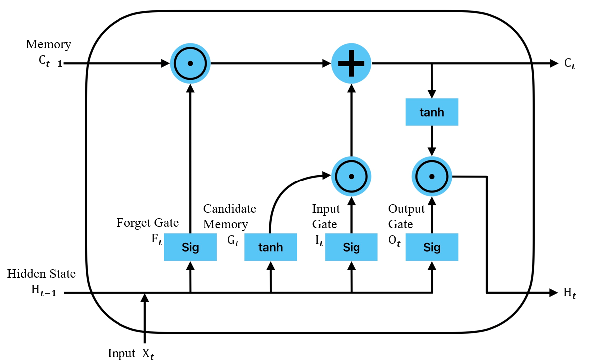
The gating mechanism of LSTM comprises three types of gates: the forgetting gate, which determines what information to discard from the cell state; the input gate, which decides what new information to add to the cell state; and the output gate, which controls the flow of information from the cell state to the next hidden state. These gates work in tandem to enable LSTMs to process long sequences efficiently, avoiding the gradient vanishing problem that is common with traditional RNNs, thus maintaining long-term information dependence.

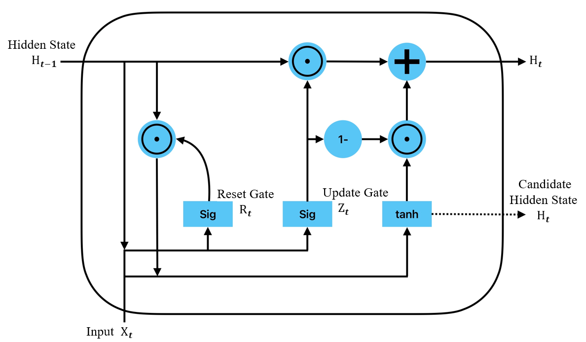
GRU simplifies the gate structure by using only two gates compared to three in LSTM: the update gate and the reset gate. The update gate determines how much of the previous memory to retain while also controlling how much new input is incorporated into the current cell state. The reset gate decides whether to disregard previous hidden states, which allows the model to reset its memory effectively, aiding in capturing relevant dependencies within the data.

Figures 1 and 2 schematically illustrate the structures of LSTM and GRU, respectively.

Figure 1. LSTM structure	Figure 2. GRU structure

3. Experimental

3.1. Experimental environment

This experiment was conducted on a computer equipped with an Intel Platinum 8352V processor, which includes 16 virtual cores, and equipped with a GeForce RTX 4090 GPU. The programming language used was Python 3.10, and the deep learning framework employed was PyTorch 2.1.0. The interactive development environment utilized for this study was JupyterLab.

3.2. Experimental data set

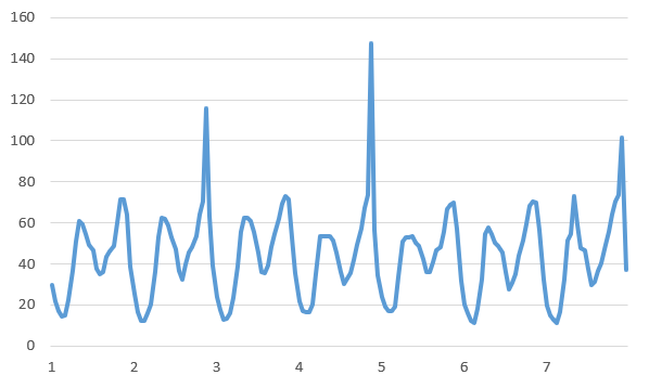
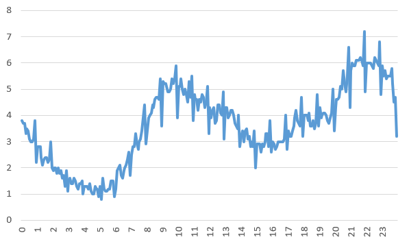
The experimental dataset used in this study was sourced from the Shenzhen Smart Meter Data Management Platform, after anonymizing the actual water consumption data from 20 residential districts in a region of Shenzhen. This dataset contains two types of readings—taken at intervals of 5 minutes and 1 hour—from 20 districts, which are classified into 20 groups according to the districts. For illustration, Fig. 3 and Fig. 4 show the hourly and five-minute water flow curves of Cell 1 for a certain week, respectively.

Figure 3. Hourly Water Volume Curve for Subarea 1	Figure 4. Water volume curve per 5 minutes for Subdivision 1

3.3. Feature extraction

To improve the prediction accuracy of XGBoost for time-series data, we extracted features from the traffic data in the original dataset and expanded the data dimensions to provide better a priori knowledge for time-series prediction. Specifically, we used the hourly dataset as the base dataset and conducted auxiliary feature extraction in terms of days and 5-minute intervals. For data pertaining to a specific day, we determined whether it was a legal holiday (including weekends), assigning the feature a value of 0 if true, and 1 otherwise. This approach provides the model with direct information about the variations in holiday activities, which aids in accurately predicting the differences in flow between holidays and weekdays. For every 5-minute water consumption data point, we applied a differential transform to find its change value, then grouped these data by hour and used K-Means for clustering. This results in identifying different change trend characteristics of water consumption per hour, such as rising then falling, falling then rising, continuously falling, or rising. These features are crucial for predicting the flow changes in the subsequent hours or even longer. The feature extraction process is illustrated in Figure 5.

Figure 5. Flowchart of feature extraction

The MSLE (Mean Squared Logarithmic Error) loss of the model after K-Means clustering at different 𝑘 values is shown in Table 2, with 𝑘=5 chosen for clustering in the experiment. The results of K-Means clustering after dimensionality reduction by PCA for the trend of hourly water flow in Cell 1 are shown in Figure 6

Table 1. MSLE Loss of the model for different values of k

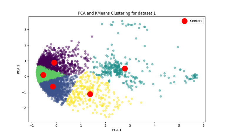
Figure 6. Clustering of Water Use Trends in Subarea 1

3.4. Assessment of indicators

Since this task is a classical regression task in machine learning, two common regression metrics, namely mean logarithmic error and mean square error, were primarily selected for evaluation in this experiment:

(1) Mean Squared Logarithmic Error (MSLE) focuses on the ratio of the predicted to true values, which can mitigate the impact of large errors and more strictly penalize the underestimation of the true value. It is especially suitable for scenarios where non-negative values are predicted, such as in water supply prediction tasks in this experiment. The calculation formula is:

\( MSLE=\frac{1}{n}\sum _{i=1}^{n} (\log{(y_{i}+1)} - \log{(\hat{y}_{i}+1)})^{2}\ \ \ (10) \)

(2) Mean Squared Error (MSE) is a widely used evaluation metric for regression tasks, assessing model performance by calculating the average of the squares of the differences between the predicted and true values. This metric is suitable for time series forecasting tasks. The formula is:

\( MSE=\frac{1}{n}\sum _{i=1}^{n} (y_{i} - \hat{y}_{i})^{2}\ \ \ (11) \)

In the above equations, \( y_i \) and \( {\hat{y}}_i \) represent the true and predicted values of the ith sample, respectively, and 𝑛 is the total number of samples.

3.5. Comparative experiments

To verify the advantages of the proposed model in terms of time series prediction accuracy, this study utilized different algorithmic models to conduct six sets of comparative experiments, employing the five-fold cross-validation method to evaluate the results based on two kinds of indicators. The results are presented in Table 1. The 1dCNN model includes three convolutional layers with convolutional kernel sizes of 9, 7, and 5, respectively. For the RNN, LSTM, and GRU models, each has three recurrent layers with 256 hidden units each.

The experimental results indicate that the K-Means + XGBoost model proposed in this paper exhibits superior performance on the time series prediction task, achieving an MSLE Loss of 0.81008.

Table 2. Comparative experimental results

3.6. Ablation experiments

The model presented in this paper incorporates holiday features from the dataset and hourly trend features clustered by K-Means, enhancing the original XGBoost model. To systematically evaluate the contribution of each feature to the prediction performance, we conducted ablation experiments by sequentially removing these features from the model and observed the specific impact on model accuracy by comparing performance before and after their removal. The results of these experiments are depicted in Table 3.

Table 3. Results of ablation experiments

From the ablation experiments, it is evident that the model which includes both the holiday feature and the water usage trend feature significantly reduces the prediction loss compared to the baseline model, which only uses the base features, and to the model which exclusively uses either the holiday or water usage trend feature. These results demonstrate that both holiday features and water usage trend features crucially enhance the accuracy of model predictions.

4. Conclusion

This paper presents a time series prediction method leveraging feature fusion and XGBoost, utilizing water consumption data from 20 neighborhoods in Shenzhen. Initially, we employ a differential transform and the K-Means algorithm to cluster finer-grained time series data, identifying and grouping changing trends into trend features. Subsequently, holiday information is integrated as an additional feature to capture anomalous behaviors and pattern changes associated with these times. Experiments demonstrate that the proposed model significantly outperforms LSTM-like methods in terms of prediction accuracy and training efficiency. Specifically, compared to LSTM, our model reduces the MSLE prediction loss by 1.42% and training time by a factor of 655.8; compared to 1dCNN, it reduces MSLE prediction loss by 8.24% and training time by a factor of 46.8. Future research directions may include exploring dynamic and adaptive clustering algorithms to address the non-stationary nature of time series data and investigating the integration of external information such as economic indicators and social events to enhance model performance.

References

[1]. Kalamara E, Turrell A, Redl C, et al. Making text count: economic forecasting using newspaper text[J]. Journal of Applied Econometrics, 2022, 37(5): 896-919.
[2]. Lam R, Sanchez-Gonzalez A, Willson M, et al. Learning skillful medium-range global weather forecasting[J]. Science, 2023, 382(6677): 1416-1421.
[3]. Sharma N, Dev J, Mangla M, et al. A heterogeneous ensemble forecasting model for disease prediction[J]. New Generation Computing, 2021: 1-15.
[4]. Box G E P, Jenkins G M, Reinsel G C, et al. Time series analysis: forecasting and control[M]. John Wiley & Sons, 2015.
[5]. Engle R F. Autoregressive conditional heteroscedasticity with estimates of the variance of United Kingdom inflation[J]. Econometrica: Journal of the econometric society, 1982: 987-1007.
[6]. Holt C C. Forecasting seasonals and trends by exponentially weighted moving averages[J]. International journal of forecasting, 2004, 20(1): 5-10.
[7]. Taylor S J, Letham B. Forecasting at scale[J]. The American Statistician, 2018, 72(1): 37-45.
[8]. Ahmadi M, Khashei M. Generalized support vector machines (GSVMs) model for real-world time series forecasting[J]. Soft Computing, 2021, 25(22): 14139-14154.
[9]. Qiu X, Zhang L, Suganthan P N, et al. Oblique random forest ensemble via least square estimation for time series forecasting[J]. Information Sciences, 2017, 420: 249-262.
[10]. Noorunnahar M, Chowdhury A H, Mila F A. A tree based eXtreme Gradient Boosting (XGBoost) machine learning model to forecast the annual rice production in Bangladesh[J]. PloS one, 2023, 18(3): e0283452.
[11]. Bhanja S, Das A. Impact of data normalization on deep neural network for time series forecasting[J]. arXiv preprint arXiv:1812.05519, 2018.
[12]. Solgi R, Loaiciga H A, Kram M. Long short-term memory neural network (LSTM-NN) for aquifer level time series forecasting using in-situ piezometric observations[J]. Journal of Hydrology, 2021, 601: 126800.
[13]. Lin H, Gharehbaghi A, Zhang Q, et al. Time series-based groundwater level forecasting using gated recurrent unit deep neural networks[J]. Engineering Applications of Computational Fluid Mechanics, 2022, 16(1): 1655-1672.
[14]. H. Steinhaus, Sur la division des corps matériels en parties, Bulletin de l'Académie Polonaise des Sciences. Classe 3 (12) (1956) 801-804. Classe 3 (12) (1956) 801-804.
[15]. S. Lloyd, Least squares quantization in PCM, in: Bell Telephone Labs Memorandum, Murray Hill NJ. Reprinted In: IEEE Trans. Information Theory IT-28 2, 1982, pp. 12-128. 1982, pp. 129-137.
[16]. R.C. Jancey, Multidimensional group analysis, Aust. J. Bot. 14 (1966) 127-130.
[17]. Chen T, Guestrin C. Xgboost: A scalable tree boosting system[C]//Proceedings of the 22nd acm sigkdd international conference on knowledge discovery and data mining. 2016: 785-794.
[18]. Hochreiter S, Schmidhuber J. Long short-term memory[J]. Neural computation, 1997, 9(8): 1735-1780.
[19]. Cho K, Van Merriënboer B, Gulcehre C, et al. Learning phrase representations using RNN encoder-decoder for statistical machine translation[J]. arXiv preprint arXiv:1406.1078, 2014.
Cite this article
Liu,C. (2024). Time-series water prediction based on feature clustering fusion and XGboost. Applied and Computational Engineering,95,86-94.
Data availability
The datasets used and/or analyzed during the current study will be available from the authors upon reasonable request.
Disclaimer/Publisher's Note
The statements, opinions and data contained in all publications are solely those of the individual author(s) and contributor(s) and not of EWA Publishing and/or the editor(s). EWA Publishing and/or the editor(s) disclaim responsibility for any injury to people or property resulting from any ideas, methods, instructions or products referred to in the content.
About volume
Volume title: Proceedings of the 6th International Conference on Computing and Data Science
© 2024 by the author(s). Licensee EWA Publishing, Oxford, UK. This article is an open access article distributed under the terms and
conditions of the Creative Commons Attribution (CC BY) license. Authors who
publish this series agree to the following terms:
1. Authors retain copyright and grant the series right of first publication with the work simultaneously licensed under a Creative Commons
Attribution License that allows others to share the work with an acknowledgment of the work's authorship and initial publication in this
series.
2. Authors are able to enter into separate, additional contractual arrangements for the non-exclusive distribution of the series's published
version of the work (e.g., post it to an institutional repository or publish it in a book), with an acknowledgment of its initial
publication in this series.
3. Authors are permitted and encouraged to post their work online (e.g., in institutional repositories or on their website) prior to and
during the submission process, as it can lead to productive exchanges, as well as earlier and greater citation of published work (See
Open access policy for details).