1. Introduction

Through the ages, the status of gold has always been high, and to some extent, gold is the world's third largest currency, its position can’t be shaken [1]. Often referred to as "safe haven" assets, according to data provided by the World Gold Council, the price of gold has grown by 8% over the past decade, which exceeds the 2% growth of global stock markets during the same period, and are seen as an important hedge against inflation, exchange rate volatility and geopolitical uncertainty. Therefore, the prediction and analysis of the gold price is also an important thing for many investors and others [2].

In the global economic integration today, the fluctuation of gold price affects the heartstring of countless investors. Both individual investors and large financial institutions have conducted in-depth research and analysis on the future trend of gold price. Therefore, for the prediction of gold prices, many scholars have launched different methodologies to reveal the different factors that affect gold prices. Such as daily charts, time series analysis, regression models, etc., or more accurate methods, without exception, to explore the uncertainty of the gold price [3]. In 2012, Tang and Xiong discussed the impact of index investment and proposed that the financialization of commodities affects the volatility of gold prices [4]. In many other factors, they can’t rely on single factor model to predict the price of gold, to emphasize the relationship between macroeconomic changes and other aspects of the birth of the multi-factor model in the gold price forecast status [5].

However, the prediction of gold prices is not so simple, and traditional methods will gradually be eliminated as time goes on. Because it is difficult to capture the complexity of gold price fluctuations and the non-linear characteristics of financial markets, it means that traditional methods will be more difficult to predict gold prices, the limitations of these approaches are becoming apparent [6]. With the advancement of science and technology, artificial intelligence, high-performance computing and other technologies are rising, deriving many algorithms that can build complex nonlinear relationships. And these advanced models will play a great potential in areas such as gold price forecasting [7].

Even though technology is advancing at a rapid pace, the volatility of the market and changes in the environment are still a challenge to predict the price of gold. Therefore, many scholars will combine the data information of gold prices in many countries and develop new methods to improve the accuracy of gold price prediction, at the same time, it is necessary to pay close attention to market dynamics and technological progress, and adjust and improve forecasting models in time [8]. Comparing the performance of Autoregressive Integrated Moving Average Mode (ARIMA) and Generalized Autoregressive Conditional Heteroskedasticity (GARCH) models in predicting gold prices, after a series of studies, scholars found that the latter is more suitable for predicting gold prices, but after improvement by Mallikar et al., showing improved accuracy of ARIMA model [9, 10]. Therefore, some scholars will use these models to calculate the rate of return on gold and then consider other factors.

This paper will use the traditional time series analysis and new algorithms for gold price prediction, which will be synthesized into a hybrid model formed by multiple methods. This model will look at a large number of factors in the movement of the gold price to provide investors and others with a method to apply to the movement of gold prices with increased accuracy, jointly promoting the healthy development of gold market.

2. Methodology

2.1. Data source

This article obtains historical data on gold prices from a number of authoritative financial data platforms, including daily price data and related macroeconomic indicators. These data platforms, including Yahoo Finance, etc., ensure the reliability of data.

2.2. Indicator selection and description

To visualize how the gold price has changed over time, this paper has plotted the gold price and its related indicators over time. This chart shows how the price of gold has fluctuated over the past 20 years. Through the time series chart, it can observe the correlation between the indicators and the gold price, so as to preliminarily judge the effectiveness of its price prediction. Figure 1 shows the highest, minimum value and annual range of gold since 2000. Since the price of gold is usually inversely correlated with the US Dollar Index, this indicator can also help investors to get an idea of the market's impact on the price of gold.

In the data preprocessing stage, it cleans and normalizes the data. Missing and outliers were removed, and the data was normalized to eliminate the impact of differences on model training (Figure 1).

In addition, the liquidation price of gold will also change depending on different factors compared to the average price at which it is sold internationally, as shown in Figure 2, where the value of gold and ounces also show a positive correlation.

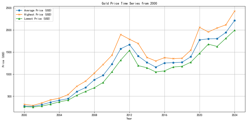
Figure 1. Gold Price Time Series from 2000.

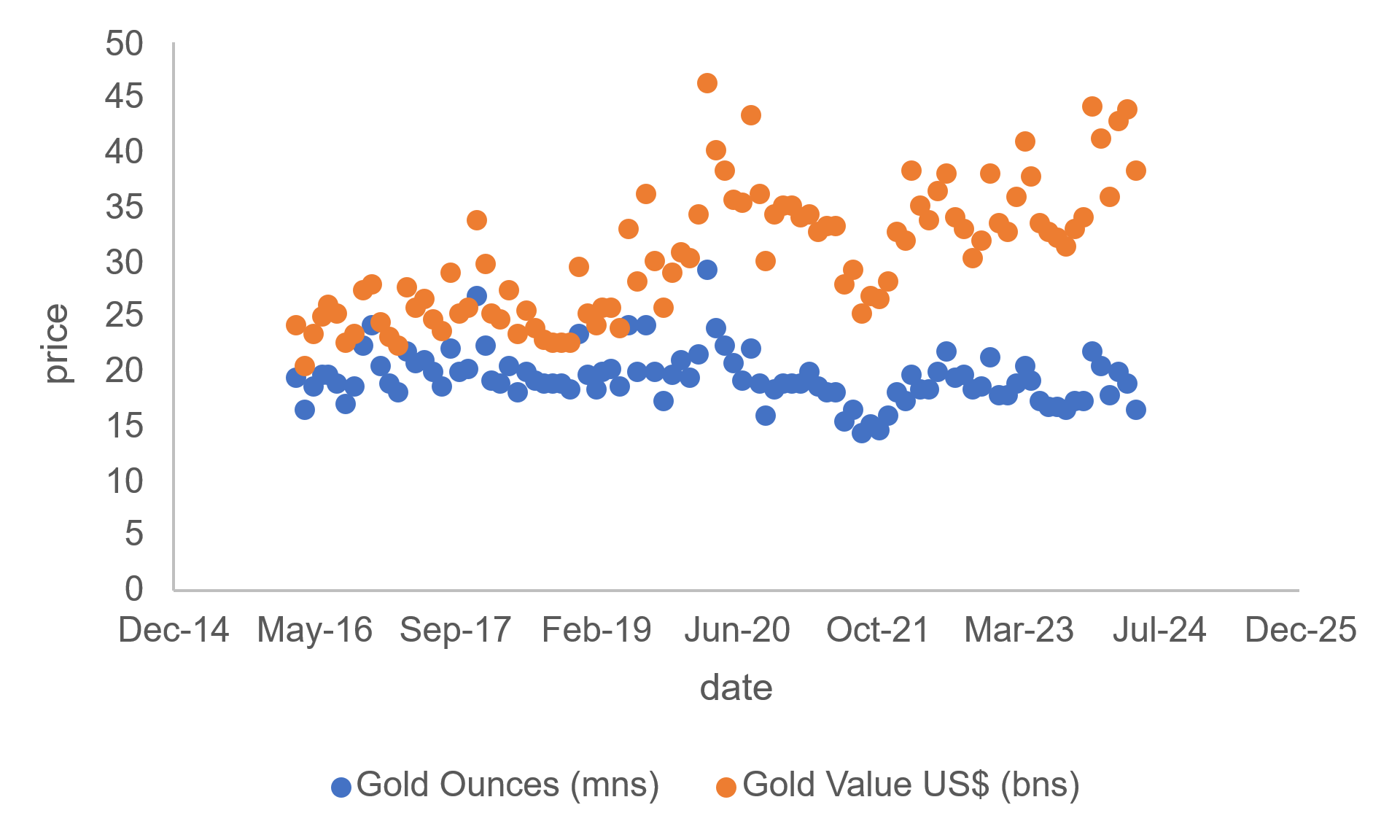
Figure 2. Gold Ounces and Gold Values in Different Time.

2.3. Method introduction

In the study on gold price prediction, it should combine time series analysis with advanced machine learning techniques to enhance forecast accuracy. The approach begins with collecting historical gold price data spanning five years, supplemented by key macroeconomic indicators such as the United States Dollar Index (USD index), US real interest rates, and Chicago Board Options Exchange Volatility Index (VIX). Data preprocessing involves thorough cleaning to remove anomalies and standardization to ensure uniformity across datasets.

Feature engineering plays a crucial role in the methodology. It extracts basic features from the raw data and compute widely-used technical indicators like moving averages, RSI, and Bollinger Bands. Additionally, it constructs new features that help capture complex market dynamics, particularly those exhibiting nonlinear relationships.

It’s necessary to select multiple machine learning models for their proven effectiveness in financial forecasting. These include linear regression for baseline comparisons, random forests for capturing nonlinear patterns, Support Vector Machines (SVMs) for robust classification, and Long Short-Term Memory networks (LSTM) networks for leveraging sequential dependencies. Each model undergoes rigorous training using cross-validation to prevent overfitting and improve generalization. Hyperparameter tuning is conducted meticulously via grid search and random search to optimize their performance.

Model evaluation is performed using established metrics such as Mean Squared Error (MSE), Root Mean Squared Error (RMSE), and the coefficient of determination (R²). These metrics provide comprehensive insights into the predictive power and goodness-of-fit of the models. Finally, the best-performing model is employed to predict future gold prices, offering valuable insights for investors and financial analysts. Through this multi-faceted approach, its aim to deliver highly accurate and reliable forecasts in the volatile gold market.

3. Results and discussion

3.1. Time series plot

First of all, the problem encountered in time series analysis is the stationarity of data. Data stationarity can be judged whether it is stationary by observing the characteristics of the data directly through the time series chart. However, the plot test has a strong subjectivity, so it will also use the ADF test, that is, the unit root test, to get a more accurate judgment, and it is necessary to perform a difference operation, so the following Figure 3 will show the results of the first differential, and its series is stable.

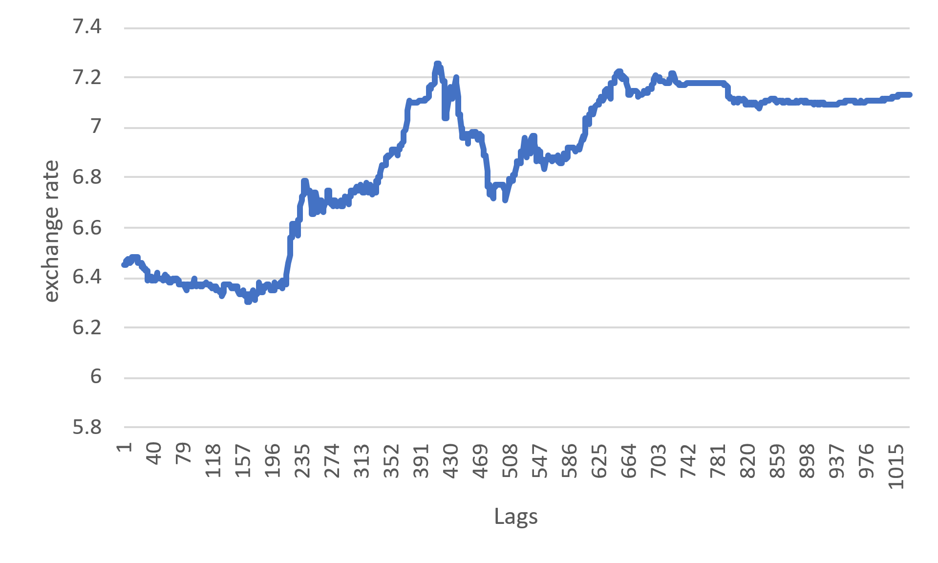
Figure 3. Timing diagram of gold price.

3.2. ADF test

To ascertain if the outcomes of the first-order differencing align with a stationary sequence, this paper employs the Augmented Dickey-Fuller (ADF) test to assess data stationarity. Its primary function is to ascertain the stationarity of the data's first differences by examining the presence of a unit root within the time series data. A unit root's existence indicates non-stationarity in the time series data; conversely, its absence suggests stationarity. The findings are illustrated in Table 1.

From the ADF test results, it can see that the original time series data is less than the 95% confidence interval ADF test value after the first-order difference processing, so the data after the first-order difference is smooth data, so the parameter 𝑑 = 1.

3.3. ACF and PACF test

Based on the stationarity test described above, it is found that the series after the first order difference is stationary, so further tests will need to be performed to ensure its accuracy.

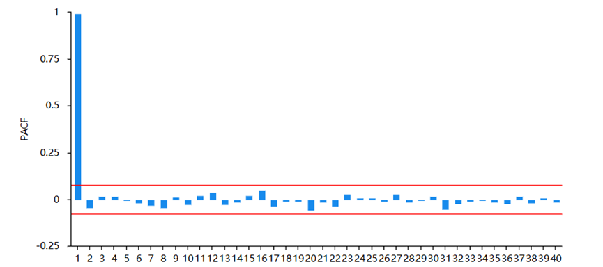
Figure 4. Results of PACF

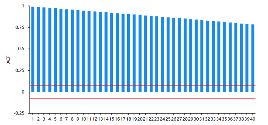
Figure 5. Results of ACF

Combined with Figure 4 and 5, the most significant order in the ACF graph can be selected as the q value, and the most significant order in the PACF can be selected as the p value; if both the ACF and PACF plots are censored, the data is white noise and is not suitable for modeling with the ARMA model. So, from the graph the author can confirm that the autoregressive order p value is 1, and the moving average order q value is 0.

3.4. ARIMA model results

Combined with the difference stage d determined in the previous step, the order of the three parameters p, d, and q has been determined, and then the ARIMA model can be established for the final detection.

Table 2. The results of fitting and predicting with the ARIMA model

From the point of view of Table 2, its true value and the fitting value and the predicted value almost coincide, so it can be determined that the model prediction results are reliable. Therefore, the ARIMA (2,1,0) model is chosen at the end of this paper.

3.5. Inferential analysis

In this paper, the author aims to explore and predict future gold price changes by building a predictive model. Specifically, the research also includes some questions. To answer these questions, it used monthly data with a time span of 5 years and chose ARIMA as the primary forecasting tool because of its demonstrated performance in handling time series data.

In the stage of model establishment and validation, it should first preprocess the data, including stationary test and seasonal decomposition. Then, using ACF and PACF diagrams to determine the parameters of the ARIMA model. By comparing different model configurations, it selects the model with the best fit. To verify the accuracy of the model, the author compared its predictions with actual prices and calculated the mean square error (MSE) and the root mean square error (RMSE). Table 3 shows the prediction results of 15 days.

4. Conclusion

This paper bases its research on the ARIMA model to predict gold prices. Through the analysis of historical gold price data, it is observed that the fluctuation of gold prices exhibits certain seasonal and trend characteristics. To capture these features, it need construct an ARIMA model and optimized its parameters. The empirical results indicate that the ARIMA model has a high degree of accuracy and reliability in predicting gold prices. By forecasting gold prices for a future period, this study provides valuable references for investors and policymakers. Moreover, this research also explores the factors influencing gold prices, such as macroeconomic conditions and monetary policy, offering a theoretical foundation and practical guidance for subsequent studies.

This paper delves into the prediction of gold prices using the ARIMA model. In the process of model construction, the non-linear and non-stationary characteristics of gold prices are fully considered. Through steps such as data preprocessing, model identification, and parameter estimation, an ARIMA model suitable for gold price prediction is successfully established. Comparative analysis with actual prices confirms the model’s advantages in terms of prediction accuracy and stability. Additionally, this study empirically analyzes the applicability of the ARIMA model in the gold market, providing beneficial decision-making references for participants in China’s gold market. However, it is worth noting that the ARIMA model has certain limitations in the prediction process, such as its weaker predictive power for extreme events. Therefore, in future research, it may be considered to combine other prediction methods to enhance the accuracy of gold price forecasting.

References

[1]. Baur D G and Lucey B M 2010 Pricing the global financial crisis: A real time test of the safe haven properties of gold. Journal of Financial Economics, 97(3), 419-442.
[2]. Narayan P K and Snaith M L 2015 Gold as a hedge against tail risk: Evidence from the US stock market. Resources Policy, 46, 102-110.
[3]. Vazquez E and Lebon F 2011 Small wavelet transform applied to short term forecasting of daily gold prices. Physic A: Statistical Mechanics and its Applications, 391(13), 3899-3908.
[4]. Tang W and Xiong J 2012 Commodity futures as an asset class: The case of index investing in China. Energy Economics, 34(6), 2013-2022.
[5]. Chen Z and Cheng L 2022 Gold price forecasting based on a SSA-ARIMA-BPNN hybrid model. HansPub, 5(2),123-135.
[6]. Diebold F X and Mariano R S 1995 Comparing Predictive Accuracy. Journal of Business and Economic Statistics, 13(3), 253-263.
[7]. Zhang Q, Li Y and Wang Y 2021 Deep hybrid neural network for precious metals price forecasting. Neurocomputing, 408, 108-120.
[8]. Johansen S and Juselius K 1990 Maximum likelihood estimation and inference on cointegration-with applications to the demand for money. Oxford Bulletin of Economics and Statistics, 52(2), 169-210.
[9]. Banu I 2012 Comparison of ARIMA and GARCH models for forecasting exchange rate movements. International Journal of Business and Social Science, 3(13).
[10]. Mallikar S and Jayalakshmi S 2014 Forecasting gold price movement using autoregressive integrated moving average (ARIMA) model with external variables. Procedia Engineering, 70, 499-506.
Cite this article
Gu,Y. (2024). Underlying factors for gold price prediction based on ARIMA models. Applied and Computational Engineering,101,147-153.
Data availability
The datasets used and/or analyzed during the current study will be available from the authors upon reasonable request.
Disclaimer/Publisher's Note
The statements, opinions and data contained in all publications are solely those of the individual author(s) and contributor(s) and not of EWA Publishing and/or the editor(s). EWA Publishing and/or the editor(s) disclaim responsibility for any injury to people or property resulting from any ideas, methods, instructions or products referred to in the content.
About volume
Volume title: Proceedings of the 2nd International Conference on Machine Learning and Automation
© 2024 by the author(s). Licensee EWA Publishing, Oxford, UK. This article is an open access article distributed under the terms and
conditions of the Creative Commons Attribution (CC BY) license. Authors who
publish this series agree to the following terms:
1. Authors retain copyright and grant the series right of first publication with the work simultaneously licensed under a Creative Commons
Attribution License that allows others to share the work with an acknowledgment of the work's authorship and initial publication in this
series.
2. Authors are able to enter into separate, additional contractual arrangements for the non-exclusive distribution of the series's published
version of the work (e.g., post it to an institutional repository or publish it in a book), with an acknowledgment of its initial
publication in this series.
3. Authors are permitted and encouraged to post their work online (e.g., in institutional repositories or on their website) prior to and
during the submission process, as it can lead to productive exchanges, as well as earlier and greater citation of published work (See
Open access policy for details).