1. Introduction

Path planning and obstacle avoidance represent significant challenges for autonomous navigation systems, which are essential for the development of self-driving cars, drone deliveries, and healthcare robots. However, there has not been much research on using Q-learning for dynamic, real-world navigation tasks. The research aims to enhance these systems through the utilization of Q-learning, a non-policy, model-free reinforcement learning algorithm initially developed by Watkins and Dayan in 1992 [1], to assist the agent in navigating a grid while avoiding specific areas. Therefore, simulations are conducted in MATLAB to train the agent in a grid environment with randomly located obstacles, and the process included setting the initial Q values of the state-action pairs, balancing exploration and exploitation using the ϵ-greedy strategy, updating the Q values with the help of environmental rewards, and evaluating the performance by means of the average path lengths, the number of collisions, and the convergence rate. The paper aims to enhance the parameters and strategies of Q-learning to increase the effectiveness of autonomous navigation systems in complex and rapidly changing environments, which can contribute to the successful development of autonomous navigation systems, and thus to the development of efficient autonomous navigation systems. Moreover, it illustrates how Q-learning can be effectively employed to regulate autonomous navigation, thus exerting a beneficial influence on the domain of reinforcement learning. The results not only provide a realistic reference for the design of more effective automatic navigation systems, but also help improve the algorithms used in self-driving cars and drones to ensure optimal functionality in different terrain conditions [2].

2. Literature Review

Q- learning is a type of reinforcement learning that does not require the model of the environment and can help an agent understand the value of actions taken in a state to get the best possible outcome. Defined by Watkins and Dayan in 1992, Q-learning stands out for its ability to approximate optimal policies even when it does not have access to an environment model [1]. The algorithm works by continuously adjusting the Q-values, which are the expected future rewards for stateaction pairs, based on the agent’s experience. This process is repeated until the Q-values represent the best policy, which helps the agent to achieve the highest total reward. The ϵ-greedy policy is typically used to control the trade-off between exploration and exploitation, allowing the agent to take new actions while also taking actions that have been known to give rewards.

When Q-learning was first introduced, it was mainly used in grid environments to tackle basic navigation and control issues. For example, Peng and Williams developed a modified Q-learning algorithm that deals with delayed rewards, bringing the algorithm closer to real-world problems [3]. The combination of Q-learning with neural networks has attracted a great deal of attention, especially after the introduction of deep Q-networks (DQNs) by Mnih et al, which integrated Q-learning with deep learning, thus enabling the algorithm to address problems with large state spaces, including those encountered in video gaming. As a result, the DQN exhibits comparable performance to humans in numerous Atari games, proving the efficiency of Q-learning in profound scenarios [2]. In addition, many extensions to the basic Q-learning algorithm have been suggested to increase its effectiveness and productivity. The overestimation problem is addressed by Double Q-learning proposed by Hasselt, which uses two Q-value estimators to enhance the stability and accuracy of the learning process [4]. Another technique proposed by Schaul et al called Prioritized Experience Replay improves the experience replay technique by sampling experiences with high potential learning rates for faster and better learning [5]. And research by Sutton and Barto emphasized the importance of reinforcement learning techniques, including Q-learning, for solving sequential decision problems [6]. It has paved the way for numerous applications in robotics, gaming, and autonomous systems. In the field of robotics, Kober et al extensively reviewed the applications of reinforcement learning in robotic control, emphasizing the potential of Q-learning for developing adaptive control policies [7]. In their study of continuous control using deep reinforcement learning, Lillicrap et al. demonstrated that Q-learning is applicable to high-dimensional action spaces, thereby extending its utility beyond discrete action environments [8].

Nevertheless, research on the use of Q-learning to solve real-world navigation problems is still not very extensive. Thus, most of them have been conducted in controlled, static environments, with fewer investigations of the issues related to the real world and its dynamic nature. This gap proves that there is more work to be done in applying Q-learning for autonomous navigation in dynamic environments, and related research has explored the application of Q-learning in environments such as self-driving cars. For example, study by Aradi on the state of the art of deep reinforcement learning in autonomous driving showcases the current advancements and challenges faced in the field [9]. Similarly, Gu et al explored the integration of reinforcement learning with computer vision techniques for autonomous navigation in complex, unstructured environments [10].

3. Methodology

3.1. Environment Setup

3.1.1. Grid-Based Environment. The grid-based environment is a two-dimensional world modelized by cells where the agent, the obstacle, and free space can be located. The goal of the agent is to move from an initial position to a target position while avoiding certain areas of the environment. The grid environment in this study is 10×10, 15×15, and 20×20 in order to examine the performance and stability of the Qlearning algorithm on different levels of problem size. Each grid cell represents a state, and the agent can move in four possible directions: up, down, left, or right.

3.1.2. Obstacle Configuration: The obstacles are distributed throughout the grid in a manner that reflects a real-world scenario. The number of obstacles is increased in proportion to the grid size in order to maintain a comparable level of difficulty across different grid sizes. For example, in a 10×10 grid, approximately half of the cells are occupied by obstacles, while in a 15×15 grid, one-third of the cells are obstacles, and in a 20×20 grid, one-fourth of the cells are obstacles. The configuration of the obstacles remains constant within an episode; however, they can be rearranged between episodes to encourage the agent to develop a general navigation strategy.

3.2. Q-Learning Algorithm Application

The Q-learning algorithms are implemented in MATLAB due to its strong numerical computing capabilities and graphical interface. MATLAB provides many libraries and simplicity, making it a suitable tool for developing and testing machine learning algorithms.

In terms of Q-value initialization, all state-action pairs have their Q-values initialized to zero. This represents an unknowing agent with no prior knowledge of the environment, which must discover the value of actions through trial and error. The Q-values are stored in a matrix with states as rows and actions as columns. In terms of the state-action selection strategy, an ϵ-greedy policy is used to balance exploration and exploitation. With probability ϵ, the agent takes a random action (explore), and with probability (1-ϵ), the agent takes the action with the highest Q-value (exploit). The exploration rate (ϵ) starts high to enable exploration and decreases over time to allow more exploitation as the agent learns about the environment. In terms of Q-value updating, the Q-values are updated iteratively using the Bellman equation:

\( Q(s,\ a)\ =\ Q(s,\ a)\ +\ \alpha\ \ast \ [r\ +\ \gamma \ \ast \ maxQ(s’, a’) — Q(s, a)] \) (1)

where s is the current state, a is the chosen action, r is the reward, s’ is the next state, \( \alpha \) is the learning rate, and γ is the discount factor. This update rule uses the agent’s experience to bring Q-values closer to expected future rewards.

3.3. Training Process in Reinforcement Learning

The training process is comprised of multiple episodes, each commencing with the agent in its initial state and concluding upon the agent’s attainment of the goal state or the maximum number of steps. In each episode, the agent selects an action in accordance with the ϵ-greedy strategy, executes the action to transition to the subsequent state and receive a reward, updates the Q-value, and then advances to the next state. This process is repeated until the Q-values have reached a state of equilibrium and the optimal values have been identified. In order to guarantee the efficacy of the training process, the following procedures were implemented. The initial step is the state resetting. At the outset of each episode, the agent is situated in the initial position, and the obstacles are relocated randomly to provide a diverse array of training scenarios. The second component is the reward function. A positive reward is conferred upon the agent upon reaching the goal, whereas a negative reward is given when the agent collides with an obstacle or is situated in a no-reward state. Upon reaching a goal, agents receive +100. Conversely, each step taken results in -1 for encouraging shorter paths. Furthermore, agents incur a negative reinforcement of -100 in the event of colliding with an obstacle. Finally, there is exploration decay. The exploration rate (ϵ) undergoes a decline over time. The exploration rate (ϵ) is initially set to 1 and then gradually decreased to 0.1, with the objective of achieving a balance between exploration and convergence to the optimal strategy.

3.4. Experiment Setup

3.4.1. Parameter Settings: The key parameters for the Q-learning algorithm are shown in Table 1. These parameters are designed to account for both the efficiency of the learning process and the speed of convergence.

Table 1. Key Parameters for the Q-Learning Algorithm

3.4.2. Training and Testing. In the training phase, the Q-learning algorithm is applied for the specified number of episodes on each grid size. The agent navigates the grid, accumulates rewards, refines Q-values, and identifies the optimal route to the objective. The efficacy of the training process is evaluated through the examination of two key metrics: the convergence of Q-values and the reduction in the number of steps required to reach the goal. In the testing phase, the learned strategy is tested by having the agent move from the starting point to the goal without updating the Q-values. The basis for performance evaluation is shown in Table 2 below.

Table 2. Basis for Performance Evaluation

Multiple trials with different obstacle layouts ensure reliability, and results are averaged to evaluate Q-learning efficiency across different grid sizes and obstacle densities. The findings inform the tuning of Q-learning parameters and the enhancement of agent mobility.

4. Results

4.1. Path-finding Visualization and Efficiency

Figure 1 below shows the path-finding results in three different grid sizes, 10×10, 15×15 and 20×20. On the smallest 10×10 grid, the Q learning algorithm shows its potential by finding a rather simple and, therefore, most efficient route to the target with the least number of deviations. This unobstructed path illustrates the algorithm’s capability for other less complicated conditions in addition to the basic navigation tasks applied in this study. For the grid size of 15×15 and 20×20, the visualization gives the impression of complex paths than the earlier sizes of the grid. The paths are extended and more complex in term of navigation, to go around a higher number of obstacles. This complexity reflects the algorithm’s ability to change its strategy when the difficulties of the environment rise and state space enlarges. In the larger grid while the algorithm still finds the target it does so through a more complex path. This efficiency in navigation even with the increase in the dimensionality is depicted towards the latter parts of Figure 1 showcasing not only the comparison of the solution between the two scales but rather the algorithms ability to achieve the goal in each and every case. This visualization serves a dual purpose. Path finding strategies at different levels of abstraction are compared and successful path optimization at each level is visualized. In addition, the flexibility of the algorithms to solve a variety of problems is demonstrated, thus emphasizing the efficiency of the algorithms to perform path finding and optimization under any conditions.

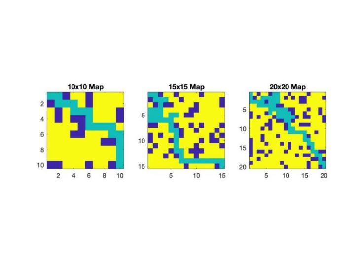
Figure 1. Path-Finding Results for 10×10, 15×15, and 20×20 Grids.

4.2. Computational Demand and Training Time

The computational time grows exponentially with the grid size, as shown in Figure 2. The smallest grids require the least amount of training time, while the largest grids require much more. This trend indicates that as task complexity increases, more computational resources are required to solve the problem, which is a major scalability issue when using Q-learning in larger, more complex scenarios.

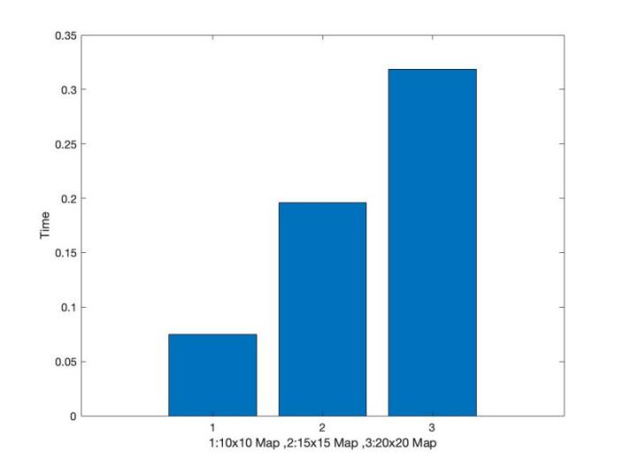
Figure 2. Comparison of Computational Time Required for Training across Different Grid Sizes.

4.3. C. Convergence Behavior

Figure 3 shows the performance of Q-learning algorithm in the convergence across the grids. It depicts the sample number needs to run the algorithm in order to achieve stable and an optimal policy. Convergence was fast in the 10×10 grid and thus the learning process was evident to be effective. On the other hand, the larger grids especially the 20×20 had a slow convergence and this could be attributed to the fact that as

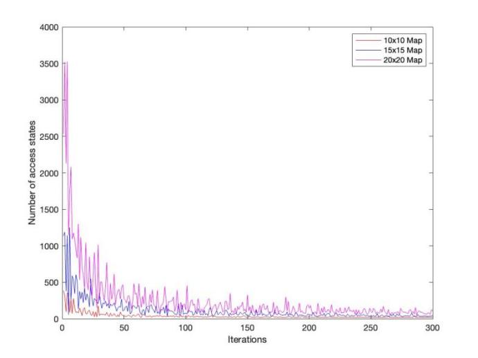
Figure 3. Convergence Behavior of Q-Learning across Various Grid Sizes

The results show that while the Q-learning algorithm can successfully learn and plan routes and strategies to traverse different environments, the complexity, computational effort, and learning rate of the paths decreases as the difficulty of the environment increases. Detailed path-finding visualizations not only help to provide a clear picture of the algorithm's performance in navigation, but can also be used to assess operational flexibility, effectiveness, and ability to handle tasks of increasing size.

5. Discussion

The results of the experimental evaluation provide insight into the efficacy and limitations of the Q-learning algorithm as the grid environment becomes increasingly complex, with one of the main issues being the increase in computational complexity when dealing with larger grids. This increase poses a significant challenge for real-time applications where timely decision making is critical. The computational cost of the algorithm also becomes higher as the grid size increases, which highlights a scalability issue that may limit its applicability in large real-world application scenarios. This study identifies several key aspects of Q-learning’s scalability and flexibility that have hitherto been given little attention in current literature. Much of the previous relevant research focuses on its applicability in limited or uncomplicated scenarios. For instance, Watkins and Dayan showed that the algorithm could efficiently solve problems and make correct choices in a grid world. However, these studies seldom addressed the issues of computational complexity and environment scaling. Thus, this study contributes to the aforementioned premises by establishing a positive correlation between the size of the environment and both computational time and learning complexity, which is a significant finding for applications that require swift decisions.

Furthermore, the ratio of exploration to exploitation is a critical parameter for the algorithm’s performance. Initially, a high exploration value allows the agent to gather general information about the environment. However, there is a crucial need to transition to exploitation during training. This transition must occur before the algorithm prematurely settles on suboptimal policies, as observed in the 20x20 grid scenario. This observation suggests that while Q-learning is efficient in navigating the environment, it may not be suited to all conditions. Adjusting exploration parameters during training could improve Q-learning’s performance on larger grids. Incorporating adaptive parameters, such as the exploration rate, or other progressive exploration methods like curiositydriven strategies, could help achieve a better balance between exploring new strategies and exploiting known ones. These improvements may address some scalability challenges, as suggested by state-of-the-art methods recommending adaptive reinforcement learning for better results in large-scale environments.

6. Conclusion

This paper presents a detailed evaluation of the Q-learning algorithm for autonomous path search on grids of different sizes (10×10, 15×15 and 20×20).The results reveal the algorithm’s capability to efficiently traverse and find optimal paths in a variety of environments, emphasizing the algorithm’s flexibility and ability to overcome various obstacles. As can be seen from the efficient direct paths in 10×10 grids, Q-learning is very effective in smaller grids, but in larger grids the scalability issues become apparent. In the 15×15 and 20×20 grids, the algorithm is still able to find the targets, albeit with longer and more complex paths than in the 10×10 grid, and with increased computational cost and time. The research reveals scalability issues that must be addressed for Q-learning to be applicable to real-world environments with multiple states and actions where timely action is important. The visualizations of path solutions allow for the observation of not only the navigation strategy employed, but also the performance of the underlying algorithm in a multitude of scenarios. The results of these visualizations are in accordance with the data regarding the computational requirements and training times for larger grids. Future research should investigate the potential of more sophisticated machine learning methods, such as deep learning or combinations of different methods, so as to enhance the efficiency of the algorithmic learning and decision-making process. Additionally, adaptive exploration and exploitation strategies can be incorporated to improve the performance of algorithms in dynamic environments.

References

[1]. Watkins, C.J.C.H. and Dayan, P. (1992) Q-Learning. Machine Learning, 8(3-4): 279-292.
[2]. Mnih, V., Kavukcuoglu, K., et al. (2015) Human-level Control through Deep Reinforcement Learning. Nature, 518: 529-533.
[3]. Peng, J. and Williams, R.J. (1993) Efficient earning and planning within the Dyna framework. Adaptive Behavior, 1(4): 437-454.
[4]. Hasselt, H. (2010) Double Q-Learning. Neural Information Processing Systems, 2613-2621.
[5]. Schaul, T., Quan, J., Antonoglou, I. and Silver, D. (2015) Prioritized Experience Replay. CoRR.
[6]. Sutton, R.S. and Barto, A.G. (1998) Reinforcement Learning: An Introduction, MIT Press.
[7]. JKober, J. Bagnell, J.A. and Peters, J. (2013) Reinforcement learning in robotics: A survey. The International Journal of Robotics Research, 32(11): 1238-1274.
[8]. Lillicrap, T.P. Hunt, J.J. Pritzel, A, et al. (2015) Continuous control with deep reinforcement learning. CoRR, abs/1509.02971.
[9]. Aradi, S. (2020) Survey of Deep Reinforcement Learning for Motion Planning of Autonomous Vehicles. IEEE Transactions on Intelligent Transportation Systems, 23(2): 740-759.
[10]. Gu, S.X., Holly, E., et al. (2017) Deep Reinforcement Learning for Robotic Manipulation with Asynchronous Off-Policy Updates. 2017 IEEE ICRA, Singapore, 3389-3396.
Cite this article
Lu,K. (2024). Route planning and obstacle avoidance using Q-Learning in MATLAB. Applied and Computational Engineering,81,112-118.
Data availability
The datasets used and/or analyzed during the current study will be available from the authors upon reasonable request.
Disclaimer/Publisher's Note
The statements, opinions and data contained in all publications are solely those of the individual author(s) and contributor(s) and not of EWA Publishing and/or the editor(s). EWA Publishing and/or the editor(s) disclaim responsibility for any injury to people or property resulting from any ideas, methods, instructions or products referred to in the content.
About volume
Volume title: Proceedings of the 2nd International Conference on Machine Learning and Automation
© 2024 by the author(s). Licensee EWA Publishing, Oxford, UK. This article is an open access article distributed under the terms and
conditions of the Creative Commons Attribution (CC BY) license. Authors who
publish this series agree to the following terms:
1. Authors retain copyright and grant the series right of first publication with the work simultaneously licensed under a Creative Commons
Attribution License that allows others to share the work with an acknowledgment of the work's authorship and initial publication in this
series.
2. Authors are able to enter into separate, additional contractual arrangements for the non-exclusive distribution of the series's published
version of the work (e.g., post it to an institutional repository or publish it in a book), with an acknowledgment of its initial
publication in this series.
3. Authors are permitted and encouraged to post their work online (e.g., in institutional repositories or on their website) prior to and
during the submission process, as it can lead to productive exchanges, as well as earlier and greater citation of published work (See
Open access policy for details).