1. Introduction

Machine learning can be thought of as: through data and algorithms, the machine learns patterns from a large amount of historical data to classify or predict new samples. The development history of machine learning can be traced back to the mid-20th century. The Turing test was developed by Alan Turing in 1950 to assess a computer's level of intelligence [1]. According to the Turing Test, a machine is considered intelligent if it can communicate with a human being and not be able to discern that it is a machine. In 1952, IBM scientist Arthur Samuel created a checkers program [2]. By watching what is currently happening, the computer program can pick up an implicit model that will help it guide future actions more effectively. The phrase "machine learning" was first used by Arthur Samuel, who defined it as a branch of research that endows computers with abilities that are not explicitly programmed. The nearest neighbor method was developed in 1967 and made it possible for computers to recognize simple patterns. [3]. The kNN algorithm's central principle is that if the majority of a sample's k nearest adjacent samples in the feature space belong to a specific category, the sample likewise belongs to that category and shares its features. In particular, Werbos introduced the multi-layer perceptron model in 1981 as part of the neural network backpropagation (BP) technique. The "decision tree" machine learning algorithm was first developed by Quinlan in 1986 [4]. Freund and Schapire introduced AdaBoost, a strong machine learning model, in 1997. The biggest feature of this algorithm is that it combines weak classifiers to form a strong classifier, and the classification effect is better than other strong classifiers. In 1995, Yan LeCun introduced the Convolutional Neural Network [5]. Influenced by biological vision systems, convolutional neural networks (CNN) commonly incorporate at least two nonlinear trainable convolutional layers, in addition to two fixed nonlinear convolutional layers. This specific configuration aims to imitate the roles of the V1 and V2 areas of the visual cortex, mirroring the functionalities of both Simple and Complex cells located within these regions. Vapnik and Cortes introduced the strong Support Vector Machine (SVM) in 1995 [6]. Breiman presented a model Random Forest in 2001 that has the ability to mix several decision trees [7]. A significant amount of input variables can be handled by random forest, which also has excellent robustness, high accuracy, a quick learning curve, and no over-fitting issues. In 2006, Hinton proposed the Deep Belief Network (DBN), opening a new era of deep learning [8]. Hinton suggested sparse coding, often known as automated coding, which involves utilizing neural networks to minimize the dimensionality of data. In 2017, Vaswani et al. proposed the Transformer model, which greatly enhanced the ability to complete tasks involving natural language processing [9].

A function's minimum value can be found using the optimization technique known as gradient descent. Its idea is to iterate along the opposite direction of the gradient of the function, thereby continuously approaching the minimum value of the function. In 1951, Herbert Robbins and Sutton Monro proposed the famous Robbins-Monro algorithm, which is the prototype of the SGD algorithm [10]. A variation of the Gradient Descent algorithm called Stochastic Gradient Descent employs only one or a small batch of data samples to calculate gradients at each iteration rather than the full training set. With the rise of deep learning, SGD has become one of the main algorithms for training large-scale neural networks. Researchers have proposed many variants of SGD (e.g., momentum method [11], Nesterov accelerated gradient (NAG) [12], Adagrad [13], Adam [14]) to solve the problems of traditional SGD in the training process.

2. Data and method

2.1. Algorithms and Model

Mini-batch SGD is a compromise between the SGD and BGD algorithms. In mini-batch SGD, a random selection of ξ data samples is used for parameter updates during gradient descent. When the dataset is large, training the algorithm is very slow. Compared to BGD, using mini-batch SGD to update parameters is faster, which helps to converge more robustly and avoid local optima. Compared to SGD, using mini-batch SGD has higher computational efficiency and can help train models more quickly. The principal formula of Mini Batch SGD is as follows:

\( {x_{t+1}}={x_{t}}-η∇F(x) \)

\( F(x)={N^{-1}}\sum _{n=1}^{N}f(x;{ξ_{n}}) \)

Here, x_t represents the model parameters, η is the learning rate, f is the loss function, and ξ is a mini-batch sample drawn from the dataset. A technique called momentum aids in suppressing oscillations and accelerating SGD in pertinent directions. Momentum SGD takes each step down as a combination of the accumulated direction from previous steps and the gradient direction at the current point. As shown in the following Fig 1 (b). In fact, a tiny bit of the update vector from the prior time step is added to the current update vector as shown in Fig. 1 [15].

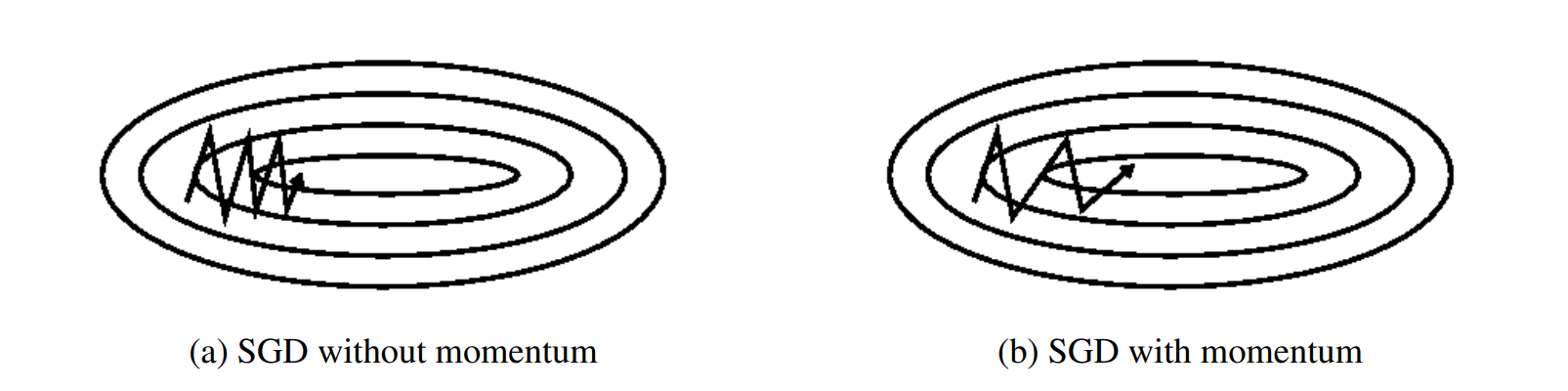
Figure 1. Comparison between SGD without and with momentum[15].

The principle formula of Momentum SGD is as follows, where v_t is the current momentum and γ is the momentum decay coefficient.

\( {X_{t+1}}={X_{t}}-{v_{t}} \)

\( {v_{t}}=γ{v_{t-1}}+η∇F(x) \)

AdaGrad is an adaptive learning rate gradient descent algorithm, proposed by Duchi et al. in 2011. This algorithm is mainly designed to address the issue of a constant learning rate in standard gradient descent algorithms. In the standard SGD algorithm, it may oscillate close to the minimum and fail to converge if the learning rate is too high; a slow pace of convergence is the result of an excessively low learning rate. The AdaGrad algorithm attempts to address this issue by adaptively changing the learning rate for each parameter. The fundamental idea behind the AdaGrad method is to adjust the learning rate of each parameter based on the sum of the squares of its prior gradients. This implies that the learning rate will be higher for features with low frequency of occurrence and lower for those with high frequency of occurrence. When dealing with sparse data, this method improves the model's performance. The principle formula of AdaGrad is as follows, where Gt is the cumulative sum of the squares of the parameter gradients, and ε is a small constant that prevents the denominator from being zero. Here, ⊙ refers to the "element-wise multiplication," also known as the Hadamard product, which is the multiplication of corresponding elements in matrices.

\( {x_{t+1}}={x_{t}}-\frac{η}{\sqrt[]{{G_{t}}-ε}}⊙∇F(x) \)

\( {G_{t,ii}}={G_{t-1,ii}}+({∇_{{θ_{i}}}}J({θ_{t,i}}){)^{2}} \)

Diederik Kingma from OpenAI and Jimmy Ba from the University of Toronto were the ones who first suggested Adam. Adam speeds up convergence by utilizing momentum and adjustable learning rates. While AdaGrad and AdaDelta add second-order momentum (second-order moment estimate) on top of SGD, SGD-M augments SGD with first-order momentum. Adam uses both first- and second-order momentum at the same time. The principle formula of Adam is as follows:

\( {x_{t+1}}={x_{t}}-\frac{η}{\sqrt[]{\hat{{v_{t}}}}+ε}\hat{{m_{t}}} \)

\( \hat{{m_{t}}}=\frac{{m_{t}}}{1-β_{1}^{t}} \)

\( \hat{{v_{t}}}=\frac{{v_{t}}}{1-β_{2}^{t}} \)

\( {m_{t}}={β_{1}}{m_{t-1}}+(1-{β_{1}})∇F(x) \)

\( {v_{t}}={β_{2}}{v_{t-1}}+(1-{β_{2}}){[∇F(x)]^{2}} \)

Here, m_t is the update for the first moment estimate (similar to momentum), vt updates the second moment estimate (uncentered variance), and β₁ and β₂ are decay rates used to adjust the importance of historical information, typically with β₁ close to 0.9 and β₂ close to 0.999. Directly utilizing mt and v_t, which are initialized to 0, will result in estimations that are skewed toward 0, particularly in the early stages. Therefore, use these two formulae for bias correction. Lastly, update the parameters using the updated first and second moment estimates.

CNNs are good at learning features that are invariant to position. In order to better capture local correlations, Kim used numerous kernels of varying sizes to extract important information from sentences while using Convolutional Neural Networks (CNN) to text classification problems. This led to the proposal of the TextCNN model. The core idea of TextCNN is to apply CNN to text classification in order to extract text features. Based on convolutional neural networks, TextCNN is a text categorization model with strong local feature extraction capabilities, a simple network topology, quick training times, and great adaptability. The architecture of the TextCNN model is fundamentally similar to that of the CNN model, consisting of an input layer, convolutional layers, pooling layers, and fully connected layers. The input layer uses a pre-trained word vector for word embedding, resulting in a final input vector dimension of: 300*128. At the same time, the emotions in Chinese text mainly appear in the form of keywords, so the size of the convolutional kernels is set to 2, 3, and 4 to capture features of the corresponding lengths.

2.2. Data and metrics

The dataset used in this experiment comes from three sources: Weibo comment sections, GitHub, and Alibaba Cloud's open-source datasets. Using web crawlers, over 20,000 text data entries were collected from Weibo comment sections. The initial goal of this experiment was to use only data from the Weibo comment section. However, after text cleaning and annotation, it was found that over 80% of the text data collected from the comment section belonged to the category of irrational thinking. Therefore, data balancing was performed on the existing data using the open-source datasets from GitHub and Alibaba Cloud. In the final dataset used for the experiment, the ratio of the three types of texts was 19983:19030:14401, totaling 53414 entries. Some data is shown in the Table 1. In this article, the model task is a three-class classification, and the confusion matrix is given in Table 2. The main evaluation metrics for the model designed in this paper are as follows:

• Cross-entropy loss function. A loss function called the cross-entropy loss function is used to evaluate how well classification models perform by comparing the actual probability distribution of the labels with the model's projected probability distribution. The calculation process is as follows:

\( Loss=-\sum _{i=1}^{M}{y_{o,i}}log{(}{P_{o,i}}),M=3,o=0,1,2 \)

• Accuracy. One of the most logical performance measures for evaluating the overall accuracy of a model's categorization choices is accuracy. It shows the percentage of accurately predicted samples out of all the samples. The calculation process is as follows:

\( Accuracy=\frac{{T_{0}}+{T_{1}}+{T_{2}}}{{T_{0}}+{T_{1}}+{T_{2}}+{F_{01}}+{F_{02}}+{F_{10}}+{F_{12}}+{F_{20}}+{F_{21}}} \)

• Training duration. Accuracy is one of the most intuitive performance metrics, used to evaluate the duration required for model training and indirectly reflecting the computational resources needed for model training.

Table 1. Examples of partial experimental data.

Table 2. Confusion matrix for this task.

3. Results and discussion

3.1. Model performance

First of all, the global learning rate set in this article is 0.01. The graphs of train loss and train accuracy are shown below. As can be seen from the Fig. 2 and Fig. 3, AdaGrad and Adam have the most stable decrease in the loss function, while mini-batch SGD has the slowest decrease in the loss function, indicating that the learning rate is too low. At the same time, the trend of train accuracy can also prove this point. The overall trends of the validation loss and validation accuracy in Fig. 4 are similar to those of the training data. At first, Adagrad was considered to be the optimal, because Adagrad has the best accuracy and the training duration is not very long. However, a very important parameter was ignored - G_t. Since G_t is the sum of squares of the gradient, G_t is a parameter that continues to increase, which directly leads to the continuous decrease of Adagrade's learning rate. Therefore, through this experimental verification, Adam performs optimally on this task, which also confirms why other models such as transformer use other variant optimizers based on the Adam algorithm. The time for different models is shown in Fig. 5.

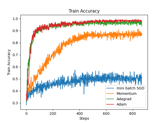
Figure 2. Train accuracy of four different optimizers (Photo/Picture credit: Original).

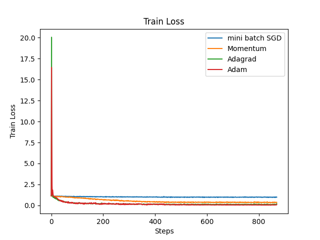
Figure 3. Train accuracy of four different optimizers (Photo/Picture credit: Original).

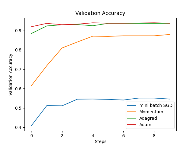
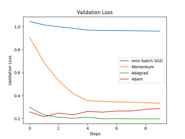
Figure 4. Validatioin accuracy (left) and loss (right) of four different optimizers (Photo/Picture credit: Original).

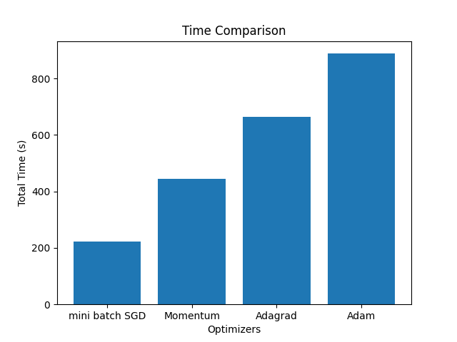
Figure 5. Train duration of four different optimizers (Photo/Picture credit: Original).

3.2. Comparison and explanation

For mini-batch SGD, it has the shortest training time, but its training accuracy is relatively low and the loss fluctuates significantly. From the formula previously, it can be seen that mini-batch SGD updates are based on only a small batch of data each time, resulting in a smaller computational load and therefore the shortest running time. However, it is precisely because only a portion of the data is used each time that the gradient estimates are unstable, resulting in significant fluctuations during parameter updates.

For momentum SGD, it has the second fastest training time, and its accuracy and loss function changes are more gradual. In fact, momentum SGD takes into account the influence of previous gradients. It builds upon mini-batch SGD by introducing "momentum" to smooth the gradient updates, thereby overcoming the gradient noise caused by small batch data and making the direction of the parameter update process more stable. At the same time, since momentum needs to be calculated, this also increases the computational workload, making the duration of momentum SGD longer than that of mini-batch SGD, but it still maintains a high level of efficiency.

For Adagrad, although it takes a longer time, the accuracy is quite high. Adagrad handles the characteristics of sparse data by adjusting the learning rate for each parameter, which allows parameters that are updated infrequently to have a larger learning rate, while parameters that are updated frequently have a smaller learning rate. Gt is the accumulation of the square of the gradient of parameter x. If the gradient of a parameter remains consistently large, the corresponding value in Gt will increase rapidly, which will reduce the effective learning rate of that parameter. On the contrary, if the gradient of a parameter is small or updates are infrequent, its corresponding Gt value increases slowly, which helps maintain a higher effective learning rate, allowing these features to receive larger updates. However, because Gt only accumulates and does not decrease, the learning rate continues to decay, causing it to drop to a very small value too early in the later stages of the learning process, leading to premature stopping of the learning. This can be verified by the trend of the loss function, which initially decreases rapidly but then significantly slows down its rate of decline at a certain point. Correspondingly, since there is a corresponding Gt for each parameter, the duration of Adagrad is relatively longer.

Adam combines concepts similar to momentum and Adagrad, providing a corresponding learning rate for each parameter. From the formula in 2.1.4, mt is the update for the first moment estimate (similar to momentum), vt updates the second moment estimate (uncentered variance), and β1 and β2 are decay rates used to adjust the importance of historical information, typically with β1 close to 0.9 and β2 close to 0.999. Since mt and vt are initialized to 0, directly using these values will lead to estimates biased towards 0, especially in the initial phase. Therefore, use these two formulas for bias correction. Finally, use the corrected first and second moment estimates to update the parameters. By introducing the parameter mt, the Adam algorithm can utilize historical gradient information to accelerate the learning process while reducing fluctuations. However, Adam's computation time is also the longest. First, Adam needs to calculate the first moment and the second moment for each parameter. Secondly, since Adam needs to simultaneously track the first and second moment estimates for each parameter, it requires more memory to store these additional data structures. Memory access and management will also significantly increase the additional time overhead, especially for the large-scale datasets are using.

3.3. For Limitations and Prospects

The goal of this article is to compare the substantial differences brought about by different optimizers and optimization algorithms through a specific task, so the choice of model is not the primary objective. Although the TextCNN model chosen for this experiment ultimately achieves an accuracy of 93%, there is still considerable room for improvement. At the same time, the results of this experiment have raised an interesting question: is the choice of model more important, or is the choice of optimization algorithm more crucial. In previous experiments, the validation accuracy achieved by the Transformer using the default optimizer was very close to the validation accuracy achieved by TextCNN using the Adam optimizer in this experiment. In the future, this experiment may further compare optimization algorithms using models such as Transformer and BERT.

4. Conclusion

By comparing relevant performance indicators and principal formulas, Adam is indeed the best optimizer under the task of this research. The text data obtained through crawler technology is used as a data set for subsequent training and verification after cleaning. At the same time, the same parameters were used to conduct a horizontal comparison of the four optimizers, including performance indicators such as accuracy, loss, and training time. It is concluded that the traditional SGD optimizer has a high dependence on the initial learning rate setting, and the optimization process is more important. Adagrad and Adam perform well under the conditions of this task, but through analysis principles, Adagrad has greater limitations. In the future, this study will continue to compare the performance of optimizers to explore optimization algorithms that can both meet accuracy requirements and save computing resources.

References

[1]. Turing A M 1950 Mind Mind vol 59(236) pp 433-460
[2]. Samuel A L 1959 Some studies in machine learning using the game of checkers IBM Journal of research and development vol 3(3) pp 210-229
[3]. Cover T and Hart P 1967 Nearest neighbor pattern classification IEEE transactions on information theory vol 13(1) pp 21-27
[4]. Quinlan J R 1986 Induction of decision trees Machine learning vol 1 pp 81-106
[5]. LeCun Y and Bengio Y 1995 Convolutional networks for images speech and time series The handbook of brain theory and neural networks vol 3361(10) p 1995
[6]. Cortes C and Vapnik V 1995 Support vector machine Machine Learning vol 20(3) pp 273-297
[7]. Breiman L 2001 Random forests Machine learning vol 45 pp 5-32
[8]. Hinton G E, Osindero S and Teh Y W 2006 A fast learning algorithm for deep belief nets Neural computation vol 18(7) pp 1527-1554
[9]. Vaswani A 2017 Attention is all you need Advances in Neural Information Processing Systems
[10]. Robbins H and Monro S 1951 A stochastic approximation method The annals of mathematical statistics pp 400-407
[11]. Qian N 1999 On the momentum term in gradient descent learning algorithms Neural networks vol 12(1) pp 145-151
[12]. Nesterov Y 2019 A method of solving a convex programming problem with convergence rate 𝑂 (1/𝑘2) Proceedings of the USSR Academy of Sciences vol 269 p 3
[13]. Duchi J, Hazan E and Singer Y 2011 Adaptive subgradient methods for online learning and stochastic optimization Journal of machine learning research vol 12 p 7
[14]. Kingma D P 2014 Adam: A method for stochastic optimization arXiv preprint arXiv:14126980
[15]. Ruder S 2016 An overview of gradient descent optimization algorithms arXiv preprint arXiv:160904747
Cite this article
Huang,W. (2024). Implementation of Parallel Optimization Algorithms for NLP: Mini-batch SGD, SGD with Momentum, AdaGrad Adam. Applied and Computational Engineering,81,226-233.
Data availability
The datasets used and/or analyzed during the current study will be available from the authors upon reasonable request.
Disclaimer/Publisher's Note
The statements, opinions and data contained in all publications are solely those of the individual author(s) and contributor(s) and not of EWA Publishing and/or the editor(s). EWA Publishing and/or the editor(s) disclaim responsibility for any injury to people or property resulting from any ideas, methods, instructions or products referred to in the content.
About volume
Volume title: Proceedings of the 2nd International Conference on Machine Learning and Automation
© 2024 by the author(s). Licensee EWA Publishing, Oxford, UK. This article is an open access article distributed under the terms and
conditions of the Creative Commons Attribution (CC BY) license. Authors who
publish this series agree to the following terms:
1. Authors retain copyright and grant the series right of first publication with the work simultaneously licensed under a Creative Commons
Attribution License that allows others to share the work with an acknowledgment of the work's authorship and initial publication in this
series.
2. Authors are able to enter into separate, additional contractual arrangements for the non-exclusive distribution of the series's published
version of the work (e.g., post it to an institutional repository or publish it in a book), with an acknowledgment of its initial
publication in this series.
3. Authors are permitted and encouraged to post their work online (e.g., in institutional repositories or on their website) prior to and
during the submission process, as it can lead to productive exchanges, as well as earlier and greater citation of published work (See
Open access policy for details).