1. Introduction

Predicting the potability of water plays a vital role in protecting public health. As an important issue at national, regional, and local levels, it necessitates the use of machine learning models to quickly and accurately access water safety.

With the development of computer technology, more advanced algorithms have been applied to water quality assessment. Models like LightGBM process continuous values through a histogram-based method, which improves training speed and is suitable for large-scale data sets. In contrast to traditional water quality assessment methods, which often rely on chemical analysis and expert judgment—processes that are typically time-consuming and costly [1]—machine learning models can analyze vast amounts of water quality data to deliver fast and accurate predictions, providing essential support for public health protection.

Machine learning models like LightGBM perform well in this field, but their complexity often makes them difficult to interpret. This paper explores the use of SHAP and LIME to enhance the interpretability of the LightGBM model on a well-trained water potability dataset. By comparing the two techniques, it aims to provide insights into which method is more effective in understanding model decisions, thereby helping to improve the transparency and credibility of model predictions [2].

2. Data Cleaning and LightGBM Model Training

2.1. Data Description

The dataset used in this study contains multiple water quality indicators, such as pH, hardness, solid content, chloramine, and sulfate, which together determine the potability of water as shown in table 1 and 2.

Table 1. Dateset

Table 2. Dateset

2.2. Data preprocessing

Data preprocessing was performed prior to training the model. First, the data were categorized into target variables and features. Missing values were then addressed by imputing the mean. The dataset was further split into training, validation, and test sets to facilitate model training, tuning, and final evaluation. Finally, in order to ensure the consistency of the data and enhance the training effect of the model, the feature data was standardized , which helped to speed up the convergence of the LightGBM model to ensure that the model can perform best on the data.

2.3. LightGBM Model Training

In this study, the LightGBM model was used to perform a binary classification task for water applications. The preprocessed dataset was divided into a training set and a validation set, where the training set was used to train the model, and the validation set was employed to monitor the model’s performance and prevent overfitting [3]. The maximum number of training rounds was set to 200 rounds and the Early Stopping mechanism was enabled. When the loss on the validation set no longer improves within 10 rounds, model training will automatically stop to prevent model overfitting.

[LightGBM] [Info] Number of positive: 785, number of negative: 1180

[LightGBM] [Info] Total Bins 2295

[LightGBM] [Info] Number of data points in the train set: 1965, number of used features: 9

[LightGBM] [Info] [binary:BoostFromScore]: pavg=0.399491 -> initscore=-0.407586

[LightGBM] [Info] Start training from score -0.407586

Training until validation scores don't improve for 10 rounds

[10] valid_0's binary_logloss: 0.609581

[20] valid_0's binary_logloss: 0.592585

[30] valid_0's binary_logloss: 0.590241

Early stopping, best iteration is:

[27] valid_0's binary_logloss: 0.58931

In the training results, the model's loss (binary logloss) on the validation set gradually decreased and reached the optimal value of 0.58931 in the 27th round. At this point, the loss on the validation set no longer decreases significantly, so the training procedure stops early at round 30.

Test Accuracy: 0.6600609756097561

Test Precision: 0.60625

Test Recall: 0.377431906614786

Test F1-Score: 0.46522781774580335

Test AUC-ROC: 0.6865997679022458

The results show that the model performs relatively consistently on the test set, especially in terms of accuracy and precision. The accuracy is 0.6601, indicating that the model can correctly predict the applicability of water in 66% of cases. However, the recall is relatively low, indicating that the model has some deficiencies in identifying positive samples (drinkable water). This means that the model may be more inclined to conservatively predict samples as negative (undrinkable).

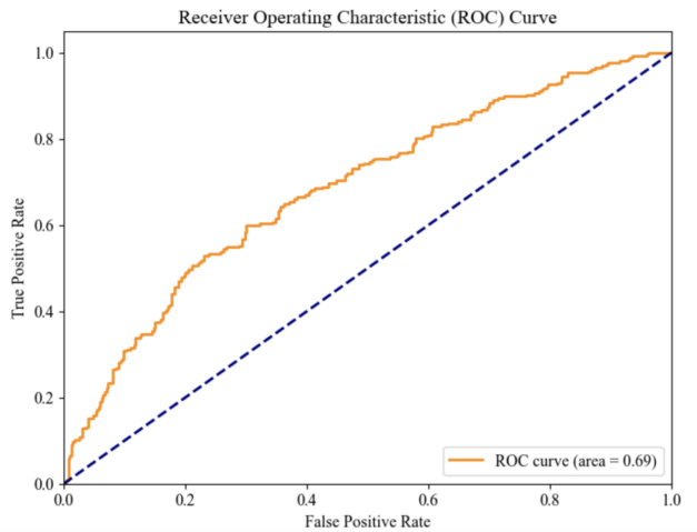
Figure 1. ROC Curve

The area under the ROC curve (AUC) is used as a performance measure of machine learning algorithms, and the ROC curve was used to evaluate the model's performance [4]. The closer the ROC curve is to the upper left corner, the better the model performs, which indicates that the model has better classification ability (Figure 1).

3. Interpretable Models

With the widespread application of machine learning, especially in complex models such as deep neural networks, random forests, and gradient boosting trees (such as LightGBM), interpretability has become an important research area. These complex models are often called "black-box models" because their decision-making process is not intuitively understandable to humans [5]. In other words, models whose internal decision-making process is difficult to explain. These models are often composed of complex mathematical operations and contain a large number of parameters and feature interactions. In order to address issues such as model transparency and credibility, interpretability tools such as SHAP (Shapley Additive Explanations) and LIME (Local Interpretable Model-agnostic Explanations) are employed to reveal the underlying principles of these black-box models, thereby facilitating greater understanding and trust in their decisions [6].

3.1. SHAP Principle

SHAP explanations, in particular, serve as a widely-used feature attribution mechanism in explainable AI. It explains the output of a machine learning model by calculating the contribution of each feature to the prediction result. The core idea of SHAP is to regard the output of the model as the payoff in a cooperative game and to distribute the contribution of each feature according to the Shapley value [7]. In game theory, the Shapley value is used to fairly distribute the total payoff in a cooperative game based on the contribution of each participant. Applying this idea to machine learning models, features are regarded as "participants", the model's prediction results are regarded as "payoffs", and the SHAP value represents the contribution of each feature to the prediction result. SHAP values ​​can explain a single prediction result and help understand the decision-making process of a specific instance. Therefore, SHAP can be applied to various machine learning models, including the LightGBM model we use.

3.1.1. Mathematical calculation principle of SHAP. SHAP value is calculated based on Shapley value, and the formula is:

\( \phi_i=\sum_{S\subseteq N\setminus{i}}\frac{|S|!\cdot(|N|−|S|−1)!}{|N|!}[v(S\cup{i})−v(S)] \)

The formula provides a method for calculating the contribution of each feature to the model’s prediction result. The calculation takes into account all possible feature combinations and averages them through weight coefficients, thereby ensuring the fairness and rationality of the formula calculation.

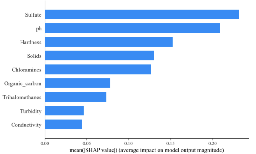
Figure 2. SHAP Model Summary

According to figure 2, which clearly shows the importance ranking of each feature in the model, Sulfate and pH are identified as the two features with the greatest impact on the model’s predictions, with their average SHAP values being significantly higher than those of other features. Analyzing the SHAP values allows for the identification of the key features influencing the prediction results, which in turn helps verify the model's validity and enhances its transparency.

3.2. LIME principle

LIME stands for "locally interpretable model-independent explanation", which is a model-independent explanation method that aims to explain the local behavior of complex models by building simplified models. The core idea of LIME is to simulate the neighborhood data around the instance around these samples to help capture the behavior of the model in the local area [8]. In fact, it is to build a simplified linear model based on these perturbed samples to approximate the decision boundary of the complex model. Linear models, such as regression models, are employed to approximate the behavior of complex models in these localized areas. LIME assumes that in the local area, the linear model can well approximate the decision boundary of the complex model. The feature weights of the linear model explain the decision of the original complex model on this instance. Finally, a visual data representation is used to demonstrate the contribution of features to the prediction result for that instance.

3.2.1. Mathematical calculation principle of LIME. The calculation formula of LIME value is:

\( \xi(x)=arg{min}_{g\in G}\mathcal{L}(f,g,\pi_x)+\mathrm{\Omega}(g) \)

The formula L(f,g,πx) represents the loss function between the original model f and the explanation model g, where πx is the weighting function of the perturbed samples in the neighborhood of sample x. And Ω(g) is to prevent the model from overfitting. Through this formula, LIME finds a simple linear model g in the local area of the complex model to approximate the behavior of the complex model f, and explains the prediction results of f by explaining the feature weights of g [9].

In this study, LIME is applied to explain the local behavior of the LightGBM model in the water potability prediction task. Specifically, LIME is applied to several key prediction samples, where perturbed samples are generated, and linear models are constructed to explain the prediction results of each sample. LIME can clearly show how the prediction of a specific water sample is affected by different water quality characteristics. For example, LIME may show that in the prediction of a non-drinkable water, "high dissolved solids content" is the main reason why the sample is classified as non-drinkable. For a water sample predicted to be drinkable, LIME can show how "moderate pH" and "low hardness" affect the model's prediction results, thereby explaining why the water sample is considered drinkable.

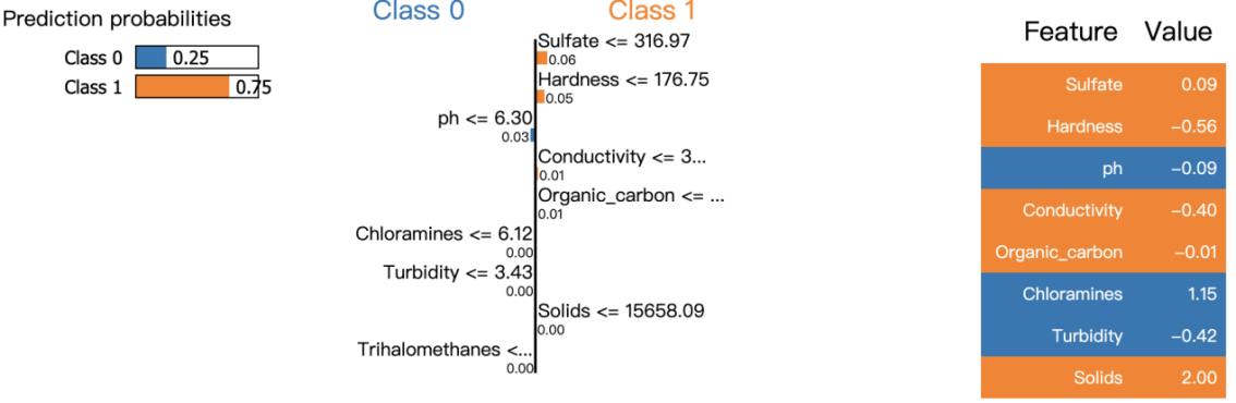
Figure 3. (From Left to Right 3.1, 3.2, 3.3): LIME Model Summary

From left to right, Figure 3.1 shows the model predicting that Class 1 (drinkable) has a 75% probability. Next, Figure 3.2 shows the contribution of each feature to the model prediction. The closer to the top, the greater the contribution. Finally, Figure 3.3 gives the specific feature values, such as a Sulfate value of 0.09 and a Hardness value of -0.56.

4. Comparative analysis of SHAP and LIME

In the study of interpretability of machine learning models, SHAP and LIME are two widely used methods. While both aim to explain the prediction process of complex models, they differ significantly in their methodologies, particularly regarding global and local interpretability [10].

4.1. SHAP's Global Interpretability Theory

The SHAP model visualization highlights the impact of key features on prediction results. From figure 4, pink points indicate a positive effect (increasing the predicted value), while blue points show a negative effect (decreasing the predicted value). Top features like "Sulfate" and "ph" exhibit both positive and negative impacts, varying across observations. Middle features like "Organic_carbon" have less impact, with more concentrated point distributions. Bottom features such as "Turbidity" and "Conductivity" contribute the least, with most impacts close to zero, indicating minimal influence on the model's predictions.

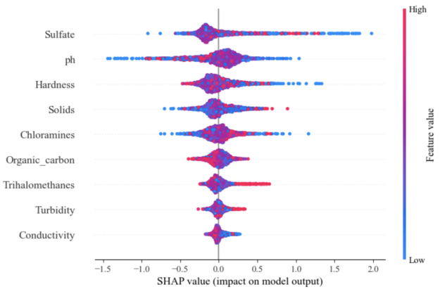
Figure 4. Impact Between SHAP Value and Feature Value

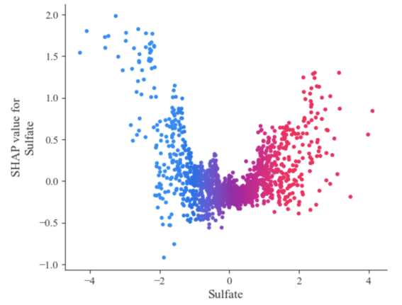
Figure 5. Relationship With SHAP Value for Sulfate

Figure 5 shows a positive relationship where higher Sulfate values (red points on the right) increase the probability of water being drinkable, while lower Sulfate values (blue points on the left) decrease this probability. The greatest impact occurs when Sulfate values are below -1 and above 1, indicating high sensitivity in these ranges. This visualization helps to understand the model's response to different Sulfate levels and allows for more targeted data collection and model adjustments.

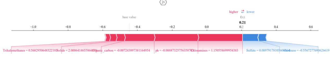
Figure 6. SHAP Force Plot

According to the force_plot (Base-value explanations) of SHAP in Figure 6, the detailed feature contributions for a single prediction are presented, with each feature’s influence on the final prediction value displayed as an arrow. The balance between positive contributions (red) and negative contributions (blue) determines the final prediction value [10].

4.2. Local Interpretability of LIME

The interpretability of the LIME model is clearly shown through its principle. The model predicts a 75% probability that this sample belongs to Class 1, indicating high confidence that the water is drinkable. The feature contribution graph reveals that features like "Sulfate" and "Hardness" support Class 1, while "Chloramines" and "Solids" lean toward Class 0. This demonstrates the model's ability to evaluate both individual feature effects and their interactions. For example, higher "Chloramines" points to Class 0, while lower "Hardness" favors Class 1. This local explanation clarifies the model's decision logic for this specific prediction.

4.3. Comparison and discussion of results

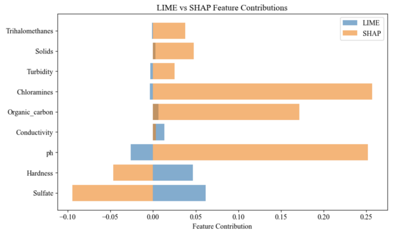
Figure 7. LIME and SHAP Model Feature Contributions

According to Figure 7, the different emphases of the two interpretation methods, LIME and SHAP, in evaluating feature contributions can be observed. For some key features, such as Sulfate and Hardness, the contribution values obtained by the two methods are relatively close, indicating that they have a relatively consistent understanding of these features, and also reflecting that the importance of these features in the model is relatively clear. However, other features (such as Chloramines and Conductivity) show obvious differences. It can be noticed that SHAP assigns significantly higher contribution values to these features compared to LIME. This difference may be due to the global consistency of SHAP, which measures the contribution of each feature by combining the interaction effects between features, while LIME focuses more on local models and may be more inclined to evaluate the impact of each feature independently of other features when interpreting [2].

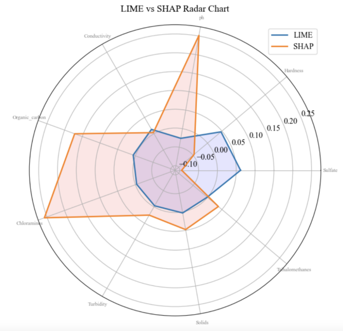
Figure 8. LIME vs SHAP Radar Chart

A radar chart (Figure 8) was created to compare SHAP’s and LIME’s contributions across different features, offering a more comprehensive perspective on model interpretation. It can be clearly seen that SHAP contributes much more to some features (such as ph) than LIME, showing that SHAP tends to give these features higher importance. This difference reflects that SHAP considers the interaction effects of features, allowing it to capture the complex effects of features globally, while LIME may show lower sensitivity to these features [11]. In addition, the more evenly distributed blue area of ​​LIME shown in the figure illustrates its conservatism and stability in local interpretation, while the orange area of SHAP reveals that it is more extensible and dynamic in global interpretation. This comparison highlights the respective strengths and limitations of SHAP and LIME. LIME is more effective in providing concise and stable local explanations, while SHAP performs better in capturing the importance and complex interactions of global features.

5. Discussion

In the wide application of machine learning, interpretability has become a key area. Interpretable models not only improve transparency and credibility, but also help practitioners understand the logic of model decisions, especially in key areas such as medicine, finance, and justice, to ensure the security and compliance of models [5]. Interpretability also helps researchers identify biases, optimize performance, and enables users to better understand the complex relationship between data and features, so as to make more informed decisions.

As mainstream model interpretation methods, SHAP and LIME each have unique advantages. SHAP provides globally consistent feature importance scores through its game theory-based framework, which is suitable for global understanding of model behavior; while LIME excels in detailed local explanations of individual predictions [11]. In the future, SHAP may focus on improving computational efficiency and adapting to complex models, while LIME can optimize in handling nonlinear feature interactions [12]. As the demand for interpretability grows, these methods may be further integrated in both theory and practice to advance model transparency and credibility.

6. Conclusion

In modern machine learning applications, interpretability has changed from an option to a necessity. This study used two maintream models, SHAP and LIME, to elucidate the decision-making process of a water quality classification model. Although SHAP demonstrates its strong ability to capture complex interactions between features and global feature importance, analysis and experimental results suggest that LIME may offer more practical advantages. LIME's flexibility and easy-to-understand local explanations make it more practical in many scenarios, and from the model results of LIME, LIME is more stable and balanced than SHAP, so LIME will make it a better choice in most applications. In the future, as the requirements for model transparency continue to increase, explanation methods such as SHAP and LIME will continue to develop to cope with more complex models and data sets. Through continuous innovation and optimization, these explanation methods can provide robust capabilities for understanding, trusting, and improving machine learning models, ultimately advancing the field of explainable AI. The rational use of these explanation methods in practical applications can not only improve the reliability and interpretability of models, but also lay the foundation for safer and more compliant AI applications.

References

[1]. Bahri, Fouad, Hakim Saibi, and Mohammed-El-Hocine Cherchali. "Characterization, classification, and determination of drinkability of some Algerian thermal waters." Arabian Journal of Geosciences 4 (2011).
[2]. Man, Xin, and Ernest Chan. "The best way to select features? comparing mda, lime, and shap." The Journal of Financial Data Science Winter 3.1 (2021): 127-139.
[3]. Ke, Guolin, et al. "Lightgbm: A highly efficient gradient boosting decision tree." Advances in neural information processing systems 30 (2017)
[4]. Bradley, Andrew P. "The use of the area under the ROC curve in the evaluation of machine learning algorithms." Pattern recognition 30.7 (1997): 1145-1159.
[5]. Li, Xuhong, et al. "Interpretable deep learning: Interpretation, interpretability, trustworthiness, and beyond." Knowledge and Information Systems 64.12 (2022): 3197-3234.
[6]. Ribeiro, Marco Tulio, Sameer Singh, and Carlos Guestrin. "" Why should i trust you?" Explaining the predictions of any classifier." Proceedings of the 22nd ACM SIGKDD international conference on knowledge discovery and data mining. 2016.
[7]. Van den Broeck, Guy, et al. "On the tractability of SHAP explanations." Journal of Artificial Intelligence Research 74 (2022): 851-886.
[8]. Shankaranarayana, Sharath M., and Davor Runje. "ALIME: Autoencoder based approach for local interpretability." Intelligent Data Engineering and Automated Learning–IDEAL 2019: 20th International Conference, Manchester, UK, November 14–16, 2019, Proceedings, Part I 20. Springer International Publishing, 2019.
[9]. Hu, Linwei, et al. "Locally interpretable models and effects based on supervised partitioning (LIME-SUP)." arXiv preprint arXiv:1806.00663 (2018).
[10]. Hasan, Md Mahmudul. "Understanding Model Predictions: A Comparative Analysis of SHAP and LIME on Various ML Algorithms." Journal of Scientific and Technological Research 5.1 (2023): 17-26.
[11]. Salih, Ahmed M., et al. "A Perspective on Explainable Artificial Intelligence Methods: SHAP and LIME." Advanced Intelligent Systems (2024): 2400304.
[12]. Aditya, P., and Mayukha Pal. "Local interpretable model agnostic shap explanations for machine learning models." arXiv preprint arXiv:2210.04533 (2022).
Cite this article
Zhang,J. (2024). Comparative Analysis of Water Applicability Predictions Explained by The LightGBM Model Using SHAP and LIME. Applied and Computational Engineering,104,151-159.
Data availability
The datasets used and/or analyzed during the current study will be available from the authors upon reasonable request.
Disclaimer/Publisher's Note
The statements, opinions and data contained in all publications are solely those of the individual author(s) and contributor(s) and not of EWA Publishing and/or the editor(s). EWA Publishing and/or the editor(s) disclaim responsibility for any injury to people or property resulting from any ideas, methods, instructions or products referred to in the content.
About volume
Volume title: Proceedings of the 2nd International Conference on Machine Learning and Automation
© 2024 by the author(s). Licensee EWA Publishing, Oxford, UK. This article is an open access article distributed under the terms and
conditions of the Creative Commons Attribution (CC BY) license. Authors who
publish this series agree to the following terms:
1. Authors retain copyright and grant the series right of first publication with the work simultaneously licensed under a Creative Commons
Attribution License that allows others to share the work with an acknowledgment of the work's authorship and initial publication in this
series.
2. Authors are able to enter into separate, additional contractual arrangements for the non-exclusive distribution of the series's published
version of the work (e.g., post it to an institutional repository or publish it in a book), with an acknowledgment of its initial
publication in this series.
3. Authors are permitted and encouraged to post their work online (e.g., in institutional repositories or on their website) prior to and
during the submission process, as it can lead to productive exchanges, as well as earlier and greater citation of published work (See
Open access policy for details).