1. Introduction

As we all know, hills and swamps cover more than 50 percent of the Earth's surface, making it difficult for wheeled and tracked machines to walk on them. In such environments, legged robots have a distinct advantage due to their legs having multiple degrees of freedom, which provides excellent adaptability and flexibility, continually inspiring research among scholars and engineers both domestically and internationally.

The first walking machine was built around 1870 by Chebyshev, based on ideas he proposed 20 years earlier. It consisted of a device based on a four-bar linkage. Using this simple mechanism, it could alternate between supporting (posture) and transferring (swing) phases[1]. Since then, quadruped robots have evolved and are now widely used in fields such as firefighting and rescue, military strategy, and aerospace.

However, the development of quadruped robots also faces numerous challenges and technical difficulties, among which gait planning plays a critical role in the stability and diversity of their movements. Gaits can be classified into three categories based on balance: static, dynamic, and quasi-static.

This article uses a legged robot with a single leg that has three degrees of freedom as an example. We analyze three types of gaits and the movement of the single leg. Then, we conduct simulations using MATLAB to verify the validity of the theoretical analysis. This supports the application of quadruped robots.

2. Static gaits

The Walk gait is the most typical gait among static gaits. When a quadruped robot moves in extremely complex environments such as stairs, obstacles, and slopes, adopting the Walk gait provides significant advantages. During locomotion, each leg of the quadruped robot has only two states: support and swing. In the Walk gait, three legs are always in the support phase. Additionally, at most only one leg can be in the swing phase. The movement sequence of the robot’s four legs in the Walk gait is left front, right rear, right front, left rear, which corresponds to 1-4-3-2 in Figure 1.

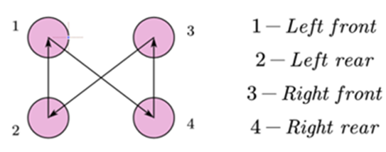
Figure 1. Diagram of the walk gait movement.

In a single movement cycle, each leg of the robot performs the same periodic motion, but the four legs have different phase relationships. The phase differences between the legs play a crucial role in the robot’s stability, efficiency, and functionality. By optimizing the phase differences, designers can enable the robot to better adapt to various application scenarios and ground conditions. Setting the phase of the left front leg to 0 (reference phase), and with the gait cycle T (the time it takes for each leg of the quadruped robot to complete one swing) set to 1, the robot's four legs' phase relationships are illustrated in Figure 2.

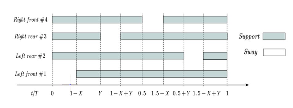
Figure 2. Diagram of the walk gait movement phases.

From Figure 2, it is evident that there are four leg support states within one movement cycle. A critical state of the Walk gait occurs when X = 0.75 and Y = 0.25. At this point, there is no distinct quadrupedal support state; only three legs are in the support phase at any given moment. The critical phase diagram of the Walk gait can be seen in Figure 3.

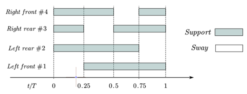
Figure 3. Critical phase diagram of the walk gait.

Under unchanged conditions, this Walk gait is theoretically the fastest among static gaits. Therefore, the Walk gait of quadruped robots is often planned according to this critical form.

3. Dynamic gaits

The Trot gait in dynamic locomotion is the most commonly used gait for quadrupeds. It is suitable for mid to low-speed running and has a relatively wide range of movement speeds. Additionally, the Trot gait offers the highest energy efficiency at moderate speeds. In the Trot gait, the quadruped robot alternates the front and rear diagonal legs touching the ground, providing good stability. Compared to other gaits, this diagonal footfall method helps maintain the robot’s balance over a larger range of speeds. The movement diagram of the Trot gait can be seen in Figure 4.

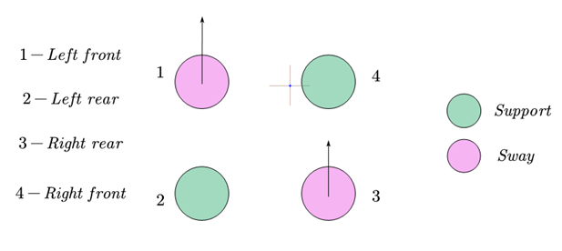
Figure 4. Diagram of the trot gait movement.

Just like the Walk gait, the Trot gait also has a phase difference between the robot's four legs, and there is a critical situation where all four legs do not simultaneously remain in the support phase. The critical phase diagram of the Trot gait can be seen in Figure 5.

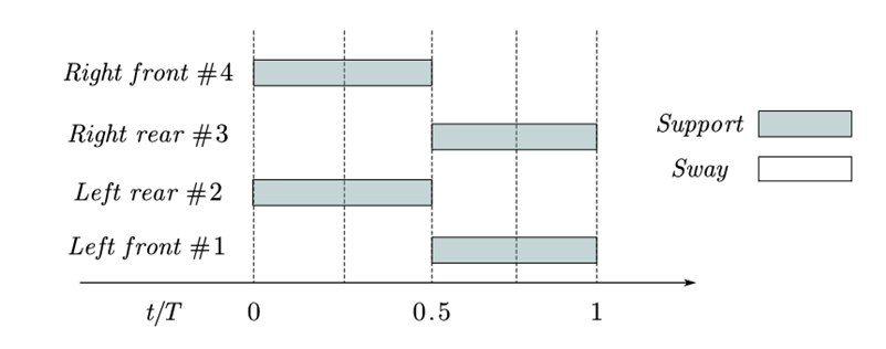
Figure 5. Critical phase diagram of the trot gait.

In an ideal situation, diagonal legs should be lifted and lowered simultaneously, which requires good synchronization and coordination performance. This depends on the precision and anti-interference capability of each leg, as well as the control strategy for coordinated movement.

In the Trot gait, the robot can adjust its stride length and frequency to adapt to different speed requirements. This flexibility allows it to cover a wide range of speeds without excessive structural adjustments. This gait utilizes elastic and inertial effects to improve energy efficiency. Under the Trot gait, the robot can partially use the elasticity of its feet for energy recovery and release, thereby maintaining high efficiency at various speeds.

4. Quasi-static gaits

The quasi-static gait of quadruped robots is a balance method that lies between static and dynamic gaits, providing a certain degree of mobility and stability. As an intermediate state, the quasi-static gait is neither completely stationary nor high-speed running; instead, it moves at a constant speed while striving to maintain body stability and reduce shaking and instability during dynamic movement. This gait enables quadruped robots to adapt well to uneven terrain while maintaining a certain speed, thereby improving motion efficiency and stability.

5. Kinematic Analysis

5.1. Kinematic forward and inverse solutions for a single leg

The forward kinematics solution for a single leg involves determining the foot endpoint position given the joint rotation angles. Establish the coordinate system shown in Figure 6.

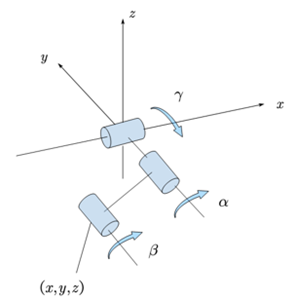
Figure 6. The coordinate system.

In Figure 6, let \( \gamma \) be the angle of rotation at the shoulder, \( \alpha \) be the angle of rotation at the thigh, and \( \beta\ \) be the angle of rotation at the calf. Let h be the length of the shoulder, hu be the length of the thigh, and hl be the length of the calf. To calculate the x, y, and z coordinates of the foot, simplify the model as shown in Figure 7.

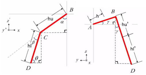
Figure 7. Simplified model[1].

As shown in Figure 7:

\( x=hu\bullet sin\alpha+hl\bullet cos\theta \) (1)

\( {hu}^{\prime\ } \) and \( {hl}^\prime\ \) are the projections of hu and hl onto the ZOY plane, respectively.

\( hu\prime=hu\bullet cos\alpha \) (2)

\( hl\prime=hl\bullet sin\theta \) (3)

\( y=h\bullet cos\gamma+(hu\prime+hl\prime)\bullet sin\gamma \) (4)

\( z=h\bullet sin\gamma+(hu\prime+hl\prime)\bullet cos\gamma \) (5)

The inverse kinematics solution for a single leg involves determining the joint angles based on known foot endpoint position. This process is closely related to the motion control of quadruped robot.

First, the angle of the lateral swing joint can be calculated according to Figure 8.

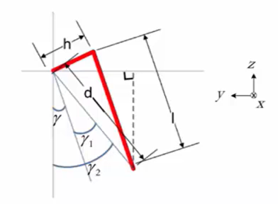
Figure 8. Simplified model [2].

\( \gamma_2= - arctan\frac{y}{z} \) (6)

\( \gamma_1= - arctan\frac{h}{l} \) (7)

\( \gamma=\gamma_2 - \gamma_1 \) (8)

Next, the angle of the hip joint can be calculated according to Figure 9.

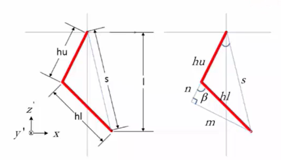
Figure 9. Simplified model[3].

\( s=\sqrt{l^2+x^2} \) (9)

\( n=\frac{s^2 - hl^2 - hu^2}{2hu} \) (10)

\( \beta= - arccos\frac{n}{hl} \) (11)

Finally, the angle of the knee joint can be calculated according to Figure 10.

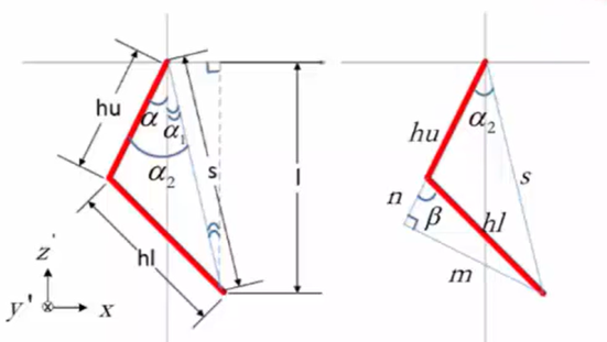
Figure 10. Simplified model [4].

\( \alpha_1= - arctan\frac{x}{l} \) (12)

\( \alpha_2=arccos\frac{hu+n}{s} \) (13)

\( {{\alpha=\alpha}_1+\alpha}_2 \) (14)

5.2. Cycloidal trajectory simulation of foot in MATLAB

In the study of quadruped robots, foot trajectory research is an important aspect. When the foot lands, it is essential to minimize instantaneous impact, ensure accurate arrival at the target point, and lift to a certain height to allow the robot to clear obstacles. To address these issues, there are various trajectory planning solutions, such as polynomial fitting, sine-cosine combinations, and optimal trajectories. This article will focus on the most common cycloid planning algorithm. The advantage of this algorithm lies in its ability to adaptively adjust the step length of the swinging trajectory according to the robot’s body speed, requiring only the input of the starting point, midpoint, and endpoint positions[5-8]. Let the current starting position of the foot be \( p_s={x_s,y_s,z_s} \) , the expected endpoint position is \( p_f={x_f,y_f,z_f} \) , the cross leg height is h, so the midpoint position is \( p_m=\frac{p_s+p_f}{2} \) .

\( x_f=\frac{1}{2}\dot{x}\bullet\mu T_s - K_{bx}({\dot{x}}_{exp} - \dot{x}) \) (15)

\( y_f=\frac{1}{2}\dot{y}\bullet\mu T_s - K_{by}({\dot{y}}_{exp} - \dot{y}) \) (16)

In the above formula, \( \ T_s \) is the gait period, and \( \mu \) is the swing phase duty cycle. By adjusting the gain parameter, it is expected that the coordinates of the landing point will change with the speed of the robot, that is, the faster the speed, the greater the stride length, and the slower the speed, the smaller the stride length[9-11]. When the speed is zero, the robot will effectively be standing still. For \( z_f \) , it can be directly equated to the current expected height of the leg: \( z_f=z_{exp} \) . The equation for the cycloidal trajectory is as follows:

\( x_{exp}=(x_f - x_s)\frac{\sigma - 2sin\sigma}{2\pi}+x_s \) (17)

\( y_{exp}=(y_f - y_s)\frac{\sigma - 2sin\sigma}{2\pi}+y_s \) (18)

\( y_{exp}=h\frac{1 - cos\sigma}{2}+z_s \) (19)

\( \sigma=\frac{2\pi t}{\mu T_s},0\text{<}t\text{<}\lambda T_s \) (20)

Let’s simulate the cycloidal trajectory in MATLAB. Setting \( p_s={ - 10, - 10,0} \) , \( p_f={40,40,z_{exp}} \) , h = 20, \( T_s=1 \) . Setting the duty cycle of the swing phase \( \mu \) = 0.5 to simulate the cycloidal trajectory of the Trot gait and \( \mu=0.25 \) to simulate the cycloidal trajectory of the Walk gait. The trajectories of both in three-dimensional space are shown in Figure 11.

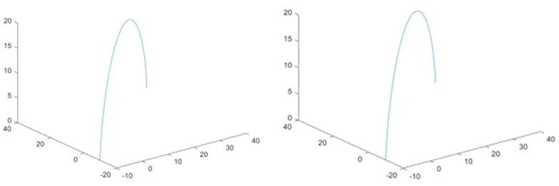
Figure 11. Cycloidal trajectories of the walk (front) and trot (back) Gaits.

The object analyzed above is the swinging leg of a quadruped robot. For the feet in the stance phase, it is necessary to use certain algorithms to adjust the joint angles in real-time, ensuring the stability of the robot’s body during movement and reducing vertical fluctuations and lateral sway. Specifically, the trajectory of the stance phase can be viewed as the path each foot of the robot follows on the ground. These paths may vary due to factors such as uneven ground and changes in the robot’s posture, but overall, they exhibit a certain regularity. This article will not introduce further here.

6. MATLAB simulation results image

Based on the above analysis, for the swing phase, first, the endpoint position of the swing leg is planned based on the robot’s real-time state estimation combined with high-level control commands. The foot movement trajectory is then calculated, and the corresponding joint angles are obtained through inverse kinematics. The entire motion process of the quadruped robot can be visualized and simulated using MATLAB. Below, the simulation process is analyzed using the Trot gait as an example. Figure 12 shows the simulation results of the Trot gait.

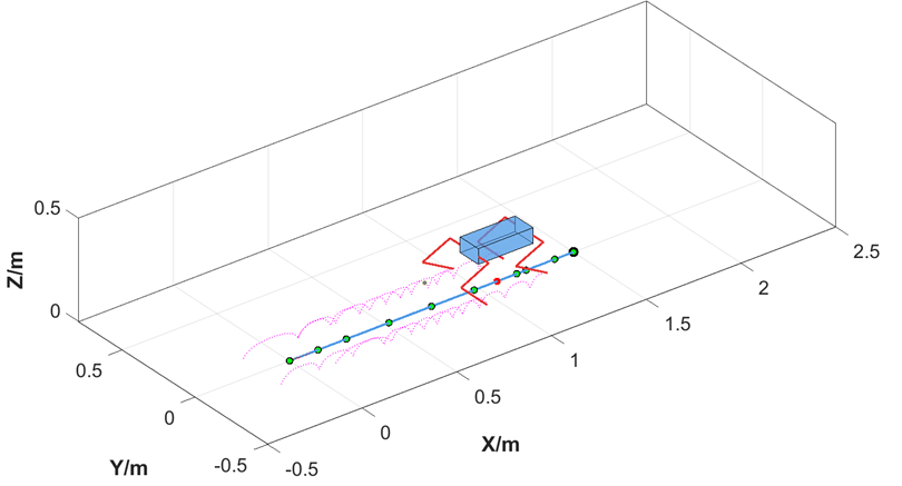
Figure 12. Simulation results of the trot gait.

While simulating the trot gait, the angular change curve of each joint can be returned, as shown in Figure 13. Since the robot is moving in a straight line, the lateral sway joint does not move, so \( \theta_1=0 \) . The angles of the hip and knee joints exhibit periodic changes, and the variation patterns between the left front leg and the right rear leg, as well as between the right front leg and the left rear leg, are identical, as \( \theta_2 \) and \( \theta_3 \) represented in Figure 13. Based on this, by taking the first and second derivatives of the angle change curves, we can obtain the angular velocity and angular acceleration curves, respectively, as shown in Figure 14.

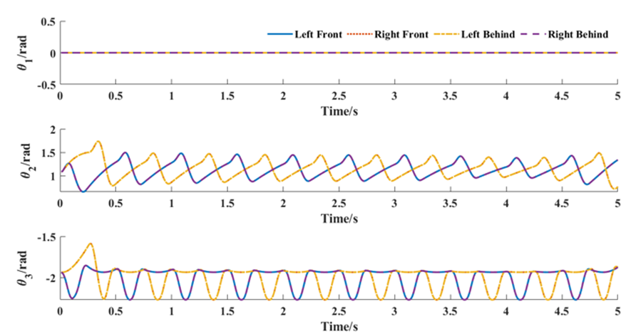
Figure 13. Curves of joint angles.

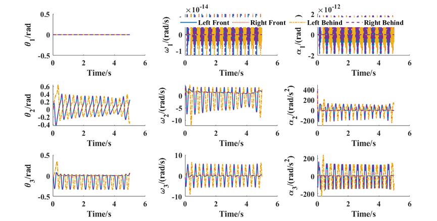
Figure 14. Curves of joint angles, angular velocities, and angular accelerations.

In the above analysis, the robot’s travel distance is set to 1.5 meters, the operating speed of the robot is 0.3 m/s, and the running time is 5 seconds. The quadruped robot can achieve relatively stable linear motion in the XOY plane using the Trot gait. At the same time, it is able to return the joint angles, angular velocities, and angular accelerations relative to the initial state during the motion process. It can be observed that these curves are basically in line with expectations.

7. Conclusion

This article analyzes the movement of a single leg based on different gait planning of quadruped robots and ultimately achieves a relatively stable Trot gait through MATLAB simulation, providing a verification of the theoretical model. With the development of today's sensor technology, on the basis of the basic motion theory of quadruped robots, quadruped robots will integrate more advanced sensing systems, such as tactile sensors and force sensors. These sensors can provide real-time feedback on ground conditions and foot contact forces, combined with various advanced algorithms for posture adjustment, helping the robot maintain stable and effective movement in various complex environments, thus enabling broader applications across different fields.

References

[1]. Zi M 2024 A Review of Quadrupeds I Current Development Status of Quadruped Robots
[2]. Sakakibara Y Kan K Hosoda Y et al 1990 Foot trajectory for a quadruped walking machine Proceedings IROS ‘90 IEEE International Workshop on July 3-6 1990 Ibaraki Japan New York NY USA IEEE pp 315-322
[3]. He D Ma P 2005 Simulation of dynamic walking of quadruped robot and analysis of walking stability Computer Simulation vol 2 pp 146-149
[4]. Li Y Li B Rong X et al 2011 Mechanical design and gait planning of a hydraulically actuated quadruped bionic robot Journal of Shandong University vol 5 pp 32-36
[5]. Pablo et al 2023 Quadruped Motion Control Technology for Quadruped Robots
[6]. Li B et al 2022 Basic Principles and Development Tutorial of Quadruped Bionic Robots
[7]. Bian Z Wang X 2021 Control Algorithms for Quadruped Robots Modeling Control and Practice
[8]. Wang P 2008 Research on Stability Walking Planning and Control Technology of Quadruped Robots Masters thesis Harbin Institute of Technology
[9]. Mok E 2023 Comprehensive Driving Planning of Quadruped Robots MATLAB and Simulink Implementation Foot End Cycloid Planning Hopf-CPG Kimura-CPG March vol 30
[10]. Mr Patrick Star 2021 Quadruped Robots – Gait Planning November vol 20
[11]. Zang F Huang M 2024 Kinematic Analysis and Gait Planning of Quadruped Robots Equipment Machinery vol 02 pp 52-55
Cite this article
Wang,Y. (2024). Quadruped Robot’s Gait Planning and Kinematic Analysis. Applied and Computational Engineering,111,17-25.
Data availability
The datasets used and/or analyzed during the current study will be available from the authors upon reasonable request.
Disclaimer/Publisher's Note
The statements, opinions and data contained in all publications are solely those of the individual author(s) and contributor(s) and not of EWA Publishing and/or the editor(s). EWA Publishing and/or the editor(s) disclaim responsibility for any injury to people or property resulting from any ideas, methods, instructions or products referred to in the content.
About volume
Volume title: Proceedings of CONF-MLA 2024 Workshop: Mastering the Art of GANs: Unleashing Creativity with Generative Adversarial Networks
© 2024 by the author(s). Licensee EWA Publishing, Oxford, UK. This article is an open access article distributed under the terms and
conditions of the Creative Commons Attribution (CC BY) license. Authors who
publish this series agree to the following terms:
1. Authors retain copyright and grant the series right of first publication with the work simultaneously licensed under a Creative Commons
Attribution License that allows others to share the work with an acknowledgment of the work's authorship and initial publication in this
series.
2. Authors are able to enter into separate, additional contractual arrangements for the non-exclusive distribution of the series's published
version of the work (e.g., post it to an institutional repository or publish it in a book), with an acknowledgment of its initial
publication in this series.
3. Authors are permitted and encouraged to post their work online (e.g., in institutional repositories or on their website) prior to and
during the submission process, as it can lead to productive exchanges, as well as earlier and greater citation of published work (See
Open access policy for details).