1. Introduction

Risk control models are tools used to identify, assess, monitor, and manage various potential risks. They are often applied in fields like finance, insurance, and corporate management to reduce the negative impact risks can have on organizations or individuals[1]. However, with the rapid development of big data and artificial intelligence technologies, traditional scoring models are facing challenges in dealing with emerging markets and economic fluctuations.

Through the logistic regression algorithm, our model will summarize the correlation between each segment of each segment of each feature of people in the dataset and the corresponding these overdue repayment behaviors, quantify the strength of this association, give a score, and finally form a set of scorecard rules for this dataset. Based on this rule, we can score customers who provide these characteristics, and these scores will be used as an important reference indicator to predict whether the customer will have untrustworthy behavior in the future.

(Background)In the financial industry, risk management is key to ensuring the stability and profitability of institutions. The scoring model is a crucial tool that provides a scientific basis for credit risk assessment by quantifying customer risk factors. This model has been widely used in areas like loan approvals and credit card issuance, significantly improving the decision-making accuracy of financial institutions[2]. This research aims to optimize the scoring model to better fit the modern financial environment.

2. Key conception and method

Analyzing the data is a critical step in generating the model, and in the process of processing the data, the meaning of certain eigenvalues (e.g., RevolvingUtilizationOfUnsecuredLines) and some artificially constructed statistics (e.g., WOE value, IV value, benchmark score, PDO) are crucial, which are basically all the model is made of.

2.1. Weight of Evidence (WOE)

WOE is a measure that converts categorical or continuous variables into a more predictive form, facilitating their interpretation and use in models[3]. WOE encodes categorical variables or bins continuous variables to establish a more direct relationship between the transformed variables and the target variable, typically a binary outcome such as default or non-default. It helps creating monotonic relationships between independent variables and the dependent variable, which is desirable in many models, especially logistic regression.

\( WOE=ln⁡(\frac{Proportion of Non\_Events in the Category}{Proportion of Events in the Category}) \)

In a later step, this value will be used to create a WOE rulebook to measure how much the value of each key feature affect the final score.

2.2. Information Value (IV)

The IV is a metric that helps evaluate the strength and importance of a predictive variable[4]. It measures how well a variable can distinguish between the two classes (e.g., default vs. non-default) in a binary classification problem. Feature selection, particularly in logistic regression models for credit scoring, often uses IV to determine which variables to include in a predictive model.

\( IV=\sum ((Proportion of Non\_Events in Category-Proporion of Events in Category)×WOE of Category) \)

2.3. Logistic regression

Logistic Regression is a widely used statistical method for binary classification problems, where the outcome can take only two possible values[5]. It is extensively applied in various fields, including credit scoring, medical diagnosis, and marketing.

Logistic regression is used to model the probability of a binary outcome based on one or more predictor variables. Unlike linear regression, which predicts a continuous outcome, logistic regression predicts the probability that a given input point belongs to a particular class.

\( P(Y=1)=\frac{1}{1+{e^{-(β0+β1X1+β2X2…+βnXn)}}} \)

P(Y=1) is the probability that the dependent variable Y equals 1.

β0​,β1​,β2​,…,βn​ are the coefficients of the model.

X1​,X2​,…, Xn​ are the independent variables.

The coefficients β are estimated using the maximum likelihood estimation (MLE) method, which finds the set of parameters that maximizes the likelihood of the observed data.

Logistic regression has various advantages in terms of interpretability, probability outputs, efficiency, lack of need for a normal distribution, and so on.

2.4. The Method of Data Binning

Data binning is a commonly used technique in data preprocessing that involves converting continuous variables into discrete variables. By dividing data into multiple intervals (or "bins"), it helps simplify the complexity of models and can also improve the performance of certain machine learning algorithms. This procedure will help to reduce the noise, handle outliers, improve model performance and enhance interpretability. For instance, in this study, all the data in the same columns with feature ”age” had been divided into 5 pieces , 0-25, 25-40, 40-50, 50-75, and above75.

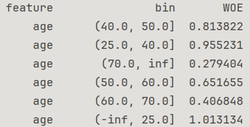
Figure 1. Bin and WOE of feature “age”

As shown in Figure 1 above, the WOE values of each bin are not too close to each other, which means these bins can obviously differ. Without the need to merge with each other, bin should be considered a success.

3. Experiments

3.1. Pretreatment

The original dataset is often poorly interpretable, and contains invalid data, missing data, which will effect the establishment of the model a lot. The preprocessing process can provide the analyst with a preliminary understanding of the data, and then solve the problem of poor interpretability of the dataset, provides convenience for further analysis and processing[6].

3.1.1. Clean up invalid data

Start by importing, the file path where the dataset is located, and a series of Python toolkits.(pandas, numpy, matplotlib, seaborn)

Through the display of the dataset by codes below, it can be found that the first column of the target table is the number of natural numbers from 0 to 149999, which is not a meaningful feature and has no practical value for model construction.

Codes:

data_path = 'data_sets/'

df_train = pd.read_csv(data_path+'cs-training.csv',sep=',')

df_test = pd.read_csv(data_path+'cs-test.csv',sep=',')

3.1.2. Processing of missing data

The following code will find the number of missing values for each column feature and its proportion to the total number of rows in the column.

Code:

null_val_sums=df_train.isnull().sum()

print(null_val_sums/df_train.shape[0])

pd.DataFrame({'Colums':null_val_sums.index,'Number of Null

Values':null_val_sums.values,'Proportion':null_val_sums.values/df_train.shape[0]})

The results are shown below. To build the model on an easily navigable dataset, the author must supplement the missing data. Calculating this ratio will give you an idea of how much of the impact of missing values will be and how to fill them, such as the NumberOfDependents column(result below), which accounts for only 2.6% of the total number of missing values, and the small impact of these gaps by replacing them with the average of all other data in the same column can be ignored. While MonthlyIncome makes up nearly 20 percent of the total, we cannot disregard it. If this feature also proves to be of sufficient value in the subsequent IV-value determination, then its large number of missing values must be taken seriously.

Result:

Monthly Income=0.198207

Number of Dependence=0.026160

[The others]=0

3.1.3. Data binning

This project's scorecard model uses WOE transformation, and data binning is a necessary condition for WOE transformation, which is also helpful for subsequent logistic regression calculations. The binning method is different for different features. Generally, after calculating the WOE value of each binning of a certain feature, you can determine whether the binning is successful by whether the WOE value between the bins is not too close. Binning is essentially an act of classification, according to the principle of classification, the WOE values in different bins should be significantly different as much as possible. (Similar WOE values can be considered for merging bins, which can improve the stability and interpretability of the model. )

Given that subsequent steps will ignore some features deemed to have a low correlation with the target SeriousDlqin2yrs, we can conclude that retesting all binning at this stage is unnecessary. Only the features judged valuable by the IV value in the next step require binning testing.

It is true that the way the binning is done can have a huge impact on the calculation of the IV values, but if the purpose is pre-processing, this level of influence does not interfere with the ability to identify features with so low IV values that they obviously do not need to be considered, as long as they are roughly in line with the basic principles of binning.

3.1.4. Calculate the IV value and retain valuable data

The data after binning can be calculated as an IV value, The IV value can be used to preliminary determine which features have high value and which should be discarded so as not to interfere with subsequent calculations. Generally, we should discard features with IV values significantly less than 0.2, retain those less than but close to 0.2 as appropriate (e.g., recalculated after strict binning), and include features greater than 0.2 in the final scorecard due to their great value. Features with IV values close to or even greater than 0.5 are very valuable and deserve attention. Occasionally, we can suspect the presence of a problem in features with IV values greater than 1 or much more than 1.

Procedure is shown in next code

Results are shown in figure2

From the results, after the lower value features are removed, there are five important features left:

Data:

age(0.2)

NumberOfTimes90DaysLate(0.49 near 0.5)

NumberOfTime60-89DaysPastDueNotWorse(0.27>0.2)

NumberOfTime30-59DaysPastDueNotWorse(0.49 near 0.5)

RevolvingUtilizationOfUnsecuredLines(1.05 above 1)

For the above five features, it is necessary to calculate their WOE values according to the principle that the WOE values between bins and bins should not be too close, strictly adjust their binning methods, and then recalculate their IV values for rigorous verification.

The data above has been adjusted by binning. There is no significant difference between the data before the adjustment.

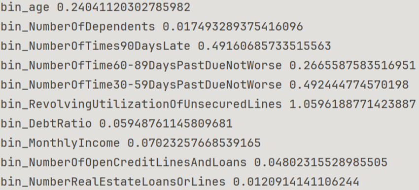
Figure 2. IV of each bin

3.2. Generate a WOE scoring booklet

The function in Figure3 summarizes the data related to the WOE value corresponding to each bin of each feature into a table (figure4), using age as an example. This table displays the total amount of data in a bin, including the number of good people (target feature SeriousDlqin2yrs=0) and the number of bad people (SeriousDlqin2yrs=1), as well as the proportion of good people and the proportion of bad people. Next, we obtain the WOE value for this bin.

We can directly obtain all bins and their corresponding WOE values to build a WOE scoring booklet, eliminating the need to visualize the data except for bin and WOE values.

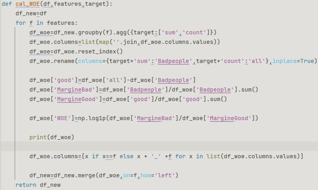
Figure 3. Calculate WOE

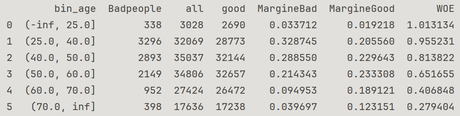
Figure 4. WOE of bin of age

This correspondence method maps the original table data into the bin, correlates each WOE value with the bin, and replaces each original table data with the corresponding WOE value. At this point, we have succeeded in standardizing the various categories of data into numerical form, which simplifies the model's input and helps the logistic regression model fit the data more accurately.

3.3. Logistic regression classification

In this program, the logistic regression model acts as a classifier to deal with binary classification problems. Specifically, Logistic Regression can help predict whether a sample is in a positive class (event, SeriousDlqin2yrs=1) or a negative class (non-event, SeriousDlqin2yrs=0) and output a probability value to measure the confidence level of the prediction, and the coefficient (weight) of each bin under each feature.

In this process, we have introduced a series of tools from the sklearn toolkit, such as train_test_split (data segmentation tool), LogisticRegression (logistic regression algorithm), accuracy_score (a measure of logistic regression accuracy), roc_auc_score (a measure of the performance of classification models, especially for binary classification problems, based on ROC function curves, and its AUC),f1_ score (harmonic average of precision and recall, model performance evaluation metric for unbalanced datasets)

Test_size=0.2 indicates a random selection of 20% of the entire dataset to assess the model's fit. We compared the model's prediction of these 20% of the data with the actual data to assess the model's accuracy.

3.3.1. Accuracy_score

Accuracy_score represents the proportion of the sample that the model predicts correctly out of the total sample:

\( Accuracy=\frac{Number of Correct Predictions}{Total Number of Predictions} \)

Accuracy_score can range from 0 to 1, with higher values indicating more accurate predictions for the model. A value of 1 indicates that the model's predictions are exactly right.

If the dataset is very unbalanced (e.g., most of the samples are in the same category), high accuracy does not necessarily mean that the model is performing well. In this case, other metrics such as F1 score, precision, and recall should be considered.

3.3.2. ROC & AUC

The AUC represents the area under the ROC curve, which ranges from 0 to 1.

AUC = 1: The model has perfect classification performance and can correctly distinguish between all positive and negative class samples.

AUC = 0.5: The model performed on par with random guesses, with no ability to classify

AUC < 0.5: The model performs poorly, and the classification is even less effective than random guessing.

ROC is an important tool to evaluate the performance of binary classification models, which describe the relationship between the false positive rate (FPR) and the true positive rate (TPR)[7].

True Percentage (TPR) also known as recall, represents the proportion of samples that are correctly classified as positive out of all positive samples.

\( TPR=\frac{TP}{TP+FN} \)

TP is the true number of cases

FN is the number of false negative cases. (True but recognized as false)

False Positive Rate (FPR) represents the proportion of all negative samples that are misclassified as positive.

\( FPR=\frac{FP}{FP+TN} \)

FP is the number of false positive cases. (False but recognized as true)

TN is the number of true and negative cases.

3.3.3. F1 score

The f1_score is a metric that assesses a classification model's performance, particularly on unbalanced datasets[8].

It is the harmonic average of precision and recall. While focusing on proper classification, we also consider the model's ability to identify minorities.

Recall is the TPR mentioned above

\( F1\_score=2*\frac{Precision*Recall}{Precision+Rrcall} \)

\( Precision=\frac{True Positives}{True Positives+False Positives} \)

The F1-score ranges from 0 to 1.

F1 = 1: Indicates that the model has the highest accuracy and recall, and the performance is perfect.

F1 = 0: Indicates that the model did not correctly predict any positive class samples.

In cases where there is an imbalance of positive and negative samples (default vs. non-default), the use of F1 score can reduce the negative impact of misclassification.

Accuracy score: 0.9736667

AUC: 0.7856135

F1: 0.202899

93.76% of the total samples were correctly predicted

The AUC value was between 0.5 and 1, which was greater than 0.75, indicating strong discrimination ability

The F1 value is only 0.2, and the accuracy and recall are generally poor.

3.4. Final scorecard

We calculate the score for each bin and feature using a logistic regression model, taking into account the model's coefficients and the WOE value of each feature. We will add these scores as a new column of data to the table in Figure 4.9, which will serve as the final scorecard.

Determine the number of points to subtract from each feature under various bins using the following formula:

\( Bin(fi)=-B * coef[i] * WOE[i] \)

B is the fractional factor, which is a constant and is used to adjust the scale of the fraction, \( B=PDO/ln(2) \)

PDO (Points to Double the Odds): Indicates how many points are added to the odds, and the odds are doubled. This parameter describes the relationship between risk and score. Common PDO values are 20, 30, 50.

The coefficient of a feature in the logistic regression model, coef[i], indicates its importance within the model. (The logistic regression model assigns a weight to each feature.)

With the above steps, the logistic regression model has summarized the due weight for each binning (coef[i]) and uses it here.

Table 1. Final Scorecard (fragment)

A is the benchmark score, usually 600 or 650 (650 is used here)

\( Score=A+bin(f1)+bin(f2)… bin(f5) \)

F1 to F5 represent the five features selected and binned above

4. Results

A scorecard model trained on 150,000 real-world samples can be used to evaluate the credit scores of customers in this dataset, and can also be used to measure the repayment risk level of other customers with corresponding data characteristics outside one or more samples. Currently, the test code supports manually entering new data in the console and generating the corresponding score immediately, however, for batch data processing, a batch of foreign data to be analyzed is also required.

The average score of the good guy is 331

The average score of the bad guys is 264

With the intermediate value of 298.5 as the boundary, it is more likely that the person corresponding to a certain score is a good person or a bad person

423>298.5

To make a judgment, the person is more likely to be a good person

5. Conclusion

This research successfully developed a robust risk control model using a scorecard based on logistic regression, providing a practical tool for assessing credit risk in financial institutions. By employing key features like Weight of Evidence (WOE) and Information Value (IV), the model effectively quantified customer risk factors, enhancing the precision of credit risk assessments. The model achieved a commendable AUC value of 0.78, indicating strong discriminatory power in distinguishing between high-risk and low-risk customers. This scorecard allows institutions to make more informed decisions in loan approvals, credit card issuance, and other credit-related services by assigning accurate scores based on customer data. The model's ability to process and analyze large datasets ensures its scalability and adaptability to different financial environments. Overall, the research provides a valuable framework for improving credit risk management, offering financial institutions a reliable and data-driven approach to predict customer behavior and manage risks effectively.

This study has also some limitations. The AUC value has only reached 0.78 at present, and there is still room for improvement

The F1score is only 0.2, which allows for optimization.

In the process of binning, the chi-square verification method can be used to further verify the rationality of binning

The performance of the model is heavily reliant on the quality and representativeness of the training data. If the dataset is biased or incomplete, the model may produce skewed results. Additionally, while IV helps in selecting important features, complex models may suffer from interpretability issues, which can be problematic in regulatory environments. Finally, the temporal validity of the model is a concern, as its predictive power may diminish over time due to changes in economic conditions, necessitating regular updates.

Further work could involve addressing these limitations by ensuring data robustness, enhancing model transparency, and establishing a framework for periodic model recalibration.

References

[1]. Allen, L., & Powell, R. (2021). Handbook of Credit Risk Management. John Wiley & Sons.
[2]. Malhotra, R., & Malhotra, D. K. (2020). "Credit Scoring Models in the Age of Big Data." Journal of Banking and Financial Technology, 4(1), 1-15.
[3]. Siddiqi, N. (2017). Intelligent Credit Scoring: Building and Implementing Better Credit Risk Scorecards. John Wiley & Sons.
[4]. Liu, S., & Shen, H. (2021). "Feature Selection for Credit Scoring Based on Information Value and Weighted Cumulative Information Value." Expert Systems with Applications, 169, 114481.
[5]. James, G., Witten, D., Hastie, T., & Tibshirani, R. (2021). An Introduction to Statistical Learning with Applications in R. Springer.
[6]. Kuhn, M., & Johnson, K. (2019). Feature Engineering and Selection: A Practical Approach for Predictive Models. CRC Press.
[7]. Chicco, D., & Jurman, G. (2020). "The Advantages of the Matthews Correlation Coefficient (MCC) over F1 Score and Accuracy in Binary Classification Evaluation." BMC Genomics, 21(1), 6.
[8]. Lipton, Z. C., Elkan, C., & Naryanaswamy, B. (2018). "Thresholding Classifiers to Maximize F1 Score." arXiv preprint arXiv:1402.1892.
Cite this article
Wang,Y. (2024). Research on the Risk Control Model Development Based on Scorecard. Applied and Computational Engineering,96,140-148.
Data availability
The datasets used and/or analyzed during the current study will be available from the authors upon reasonable request.
Disclaimer/Publisher's Note
The statements, opinions and data contained in all publications are solely those of the individual author(s) and contributor(s) and not of EWA Publishing and/or the editor(s). EWA Publishing and/or the editor(s) disclaim responsibility for any injury to people or property resulting from any ideas, methods, instructions or products referred to in the content.
About volume
Volume title: Proceedings of the 2nd International Conference on Machine Learning and Automation
© 2024 by the author(s). Licensee EWA Publishing, Oxford, UK. This article is an open access article distributed under the terms and
conditions of the Creative Commons Attribution (CC BY) license. Authors who
publish this series agree to the following terms:
1. Authors retain copyright and grant the series right of first publication with the work simultaneously licensed under a Creative Commons
Attribution License that allows others to share the work with an acknowledgment of the work's authorship and initial publication in this
series.
2. Authors are able to enter into separate, additional contractual arrangements for the non-exclusive distribution of the series's published
version of the work (e.g., post it to an institutional repository or publish it in a book), with an acknowledgment of its initial
publication in this series.
3. Authors are permitted and encouraged to post their work online (e.g., in institutional repositories or on their website) prior to and
during the submission process, as it can lead to productive exchanges, as well as earlier and greater citation of published work (See
Open access policy for details).