1. Introduction

Credit scoring models play a crucial role in modern financial systems, enabling institutions to assess the risk associated with lending decisions. The development of these models has been driven by the increasing demand for effective tools to predict the likelihood of a borrower defaulting on a loan. FICO scores, for instance, have been widely adopted as a key metric in credit risk management, allowing lenders to make informed decisions about creditworthiness [1]. These models not only benefit financial institutions by mitigating risk but also help borrowers access loans under better terms, thus improving financial inclusion [2]. The application of machine learning techniques in credit scoring has gained significant traction in recent years. Logistic regression has historically been the standard model used for credit scoring because of its simplicity and interpretability [3]. However, advancements in machine learning, including the use of random forests and gradient boosting machines, have opened new avenues for enhancing model accuracy [4]. These models are particularly effective in handling large, complex datasets and capturing non-linear relationships that traditional statistical methods may overlook [5]. Data preprocessing and feature engineering play an essential role in building robust credit scoring models. Missing data, for example, is a common issue in real-world datasets, and the choice of imputation method can significantly impact model performance. Research shows that random forest imputation is a powerful non-parametric method for handling missing values, especially in datasets containing mixed-type variables [6]. Furthermore, binning techniques and the calculation of Weight of Evidence (WoE) are often used to convert continuous variables into categorical ones, making them more suitable for model training [7]. The model evaluation phase is equally important in ensuring the reliability of a credit scoring model. Area Under the ROC Curve (AUC) has become a standard metric for evaluating binary classification models, such as those used in credit scoring. A high AUC score indicates that the model is highly capable of distinguishing between good and bad credit risks [8]. Additionally, the model's performance should be validated using out-of-sample testing to avoid overfitting, which is a common problem in machine learning applications [9]. In recent years, the integration of alternative data sources, such as social media activity and e-commerce behavior, into credit scoring models has been explored as a way to enhance predictive power [10]. These new data sources provide deeper insights into consumer behavior, enabling lenders to make more informed decisions, particularly in cases where traditional credit data may be sparse or unavailable.

2. Research Methodology

As shown in Figure 1, the design process for this project involved several key steps, including data preprocessing, feature engineering, model training, and model evaluation.

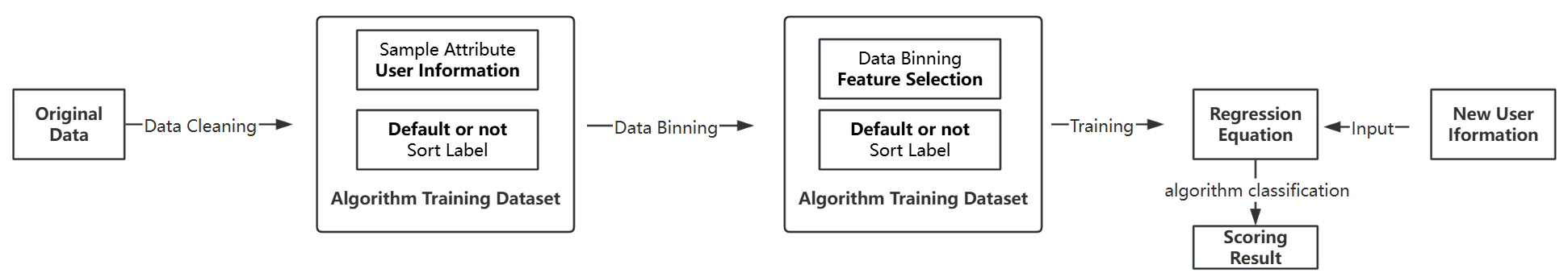
Figure 1. Process of FICO Scoring

As a classic binary classification algorithm, logistic regression is widely used in the construction of credit scores, especially in dealing with the binary classification problem of “default” and “non-default” [11]. Compared with the traditional linear regression model, logistic regression can better capture the probabilistic characteristics of credit risk and has become a standard tool in risk assessment [12]. Since credit scoring is a numerical value, and the binary classification label is a discrete quantity like “normal/default,” it is necessary to use the Sigmoid function in logistic regression:

\( y = \begin{cases}0,when\frac{1}{1+{e^{-({a_{1}}{x_{1}}+{a_{1}}{x_{2}}+…+b)}}} \lt 0.5 \\ 0/1,when\frac{1}{1+{e^{-({a_{1}}{x_{1}}+{a_{1}}{x_{2}}+…+b)}}}=0.5 \\ 1,when\frac{1}{1+{e^{-({a_{1}}{x_{1}}+{a_{1}}{x_{2}}+…+b)}}} \gt 0.5\end{cases} \) (1)

Convert the result of comparing the continuous value with the threshold into a discrete classification label. Based on this, this text obtains the expression used for calculating the credit score.

2.1. Data Processing

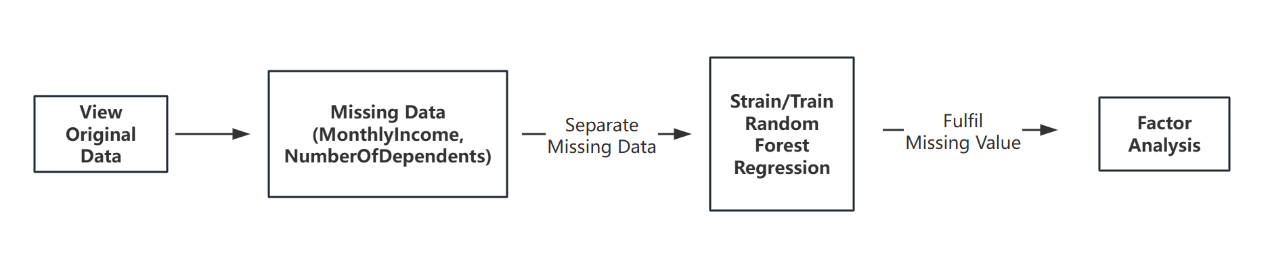
Figure 2. Process of data cleaning

Figure 2 shows the dataset contained missing values, particularly in fields like Monthly Income and Number of Dependents. Missing data is a common problem in credit scoring models. In order to ensure the integrity of the data, the paper used a random forest regression model to fill in the missing values. It has been shown that the random forest algorithm provides high accuracy when dealing with mixed data types and has been successfully applied in the field of credit risk assessment [13]. Missing values were imputed using a Random Forest regressor to ensure the model had a complete dataset for training.

Additionally, outliers in the dataset were handled using custom functions to remove extreme values, allowing the model to focus on realistic data points. Binning was used to group similar values for key features, simplifying the input data for the model.

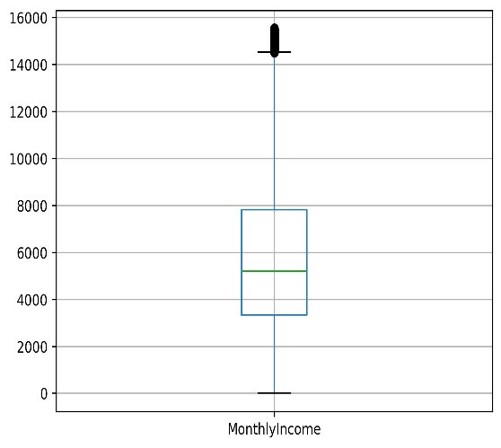
Figure 3. Original Distribution of Outliers (Monthlyincome)

Figure 3 shows a skewed MonthlyIncome distribution, with most incomes between 3000 and 7000, a median slightly above 4000, and several high-income outliers exceeding 14,000.

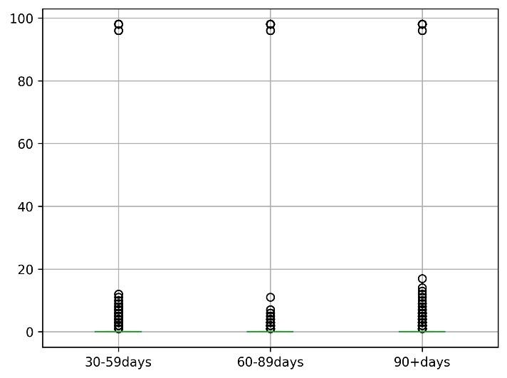
Figure 4. The Original Distribution of Three Attributes

Figure 4 shows the original distribution of number of defaults over the past 30-59, 60-89, 90+ days, and after deleting the outliers, the distribution is shown in Figure 5.

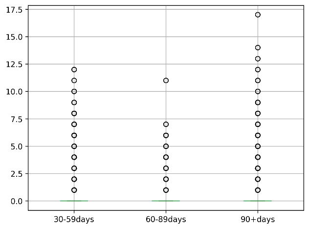
Figure 5. The Distribution of Three Attributes after Removing Outliers

2.2. Feature Engineering

Feature engineering is critical in building an effective predictive model. This text, calculated Weight of Evidence (WoE) and Information Value (IV) for each feature to evaluate their importance in predicting default risk. In the feature engineering stage, WoE and Information IV are commonly used feature selection tools, especially in credit risk modeling, where they are effective in improving the predictive performance of the model [14]. These methods transform raw data into a form more suitable for model training and increase the sensitivity of the model to default risk. The formula for WoE (Weight of Evidence) is:

\( WoE=ln(\frac{Good Distribution Percentage}{Bad Distribution Percentage}) \) (2)

The formula for IV (Information Value) is:

\( IV=∑(WoE×(Good Percentage-Bad Percentage))\ \ \ （3） \)

The Graph of the Calculated Information Value:

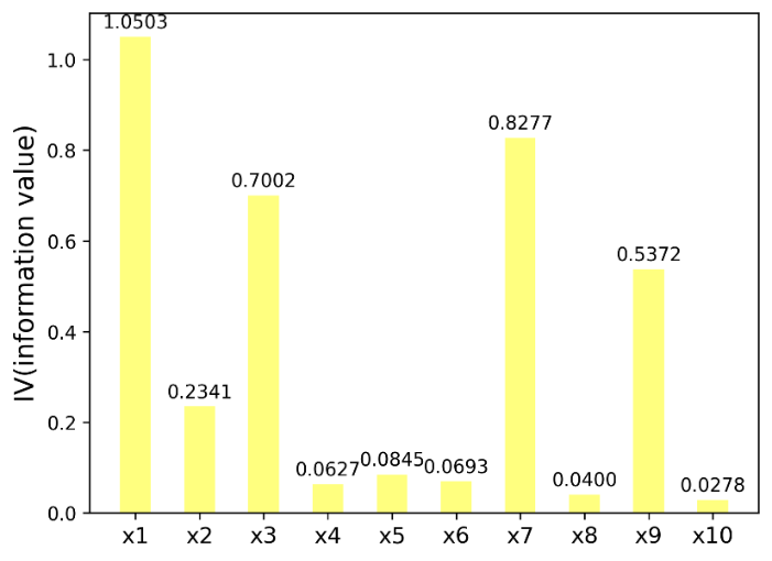
Figure 6. Information Value

Figure 6 represents the distribution of information values for different variables. The x-axis shows the variables, while the y-axis indicates the corresponding information value. Each bar in the histogram corresponds to a specific variable and its associated information value.

2.3. Model Training

For model training, a logistic regression model was chosen. Logistic regression is well-suited for binary classification problems like default prediction, where the output is a probability between 0 and 1. The sigmoid function was used to map the linear regression output to a range of probabilities, making it ideal for credit risk analysis.

The formula for logistic regression is:

\( P(y=1X)=\frac{1}{1+{e^{-({β_{0}}+{β_{1}}{X_{1}}+{β_{2}}{X_{2}}+…+{β_{n}}{X_{n}})}}}\ \ \ (4) \)

Where \( {β_{0}} \) is the intercept, and \( {β_{1}},{β_{2}},...,{β_{n}} \) are the coefficients for the input features \( {X_{1}},{X_{2}},...,{X_{n}} \)

To enhance model performance, the features were transformed into WoE values, using a custom `get_woe` function. The training set and test set were processed to convert raw features into these WoE values, which improved the model’s ability to generalize to unseen data.

At the same time, regularization is used to prevent overfitting, with \( samples \) , the loss function of linear regression is:

\( L(w)=\frac{1}{2}\sum _{i=1}^{m} ({f_{w}}({x_{i}})-{y_{i}}{)^{2}} \\ =\frac{1}{2}\sum _{i=1}^{m} ({w^{⊤}}{x_{i}}-{y_{i}}{)^{2}}\ \ \ （5） \)

Based on the above formula, add a regularization term to obtain a new loss function:

\( L(w)=\frac{1}{2}(\sum _{i=1}^{m} ({w^{⊤}}{x_{i}}-{y_{i}}{)^{2}}+λ\sum _{j=1}^{n} w_{j}^{2})\ \ \ （6） \)

Intuitively, when minimize this new loss function, on one hand, researchers want to minimize the error term \( \sum _{i=1}^{m} ({w^{⊤}}{x_{i}}-{y_{i}}{)^{2}} \) of the linear regression itself. On the other hand, the parameters shouldn't be too large, otherwise the regularization term \( λ\sum _{j=1}^{n} w_{j}^{2} \) will become large. The regularization term, also called the penalty term, is used to penalize the model for becoming too complex due to excessively large weights \( λ\sum _{j=1}^{n} w_{j}^{2} \) . The parameter \( λ \) in the regularization term is used to balance the loss function and the regularization term, and is known as the regularization coefficient. The larger the coefficient, the stronger the penalty effect of the regularization term.

Figure 7 shows the Normal/Default Customer Score Distribution, and there are 3 features:

Overlapping Distributions: There is some overlap between the two distributions in the range of scores between 500 and 600, which suggests that distinguishing between "normal" and "charged" cases in this range may be challenging, as both categories exhibit similar probabilities.

Separation of Categories: After a score of approximately 600, the dashed blue line (charged) peaks higher than the solid orange line (normal), implying that at higher scores, "charged" cases are more probable. Score Ranges: For scores below 500, the probability of "normal" cases (orange line) is higher, suggesting that low scores are more associated with normal cases. On the other hand, higher scores (600+) are more likely to be associated with "charged" cases, as indicated by the blue line's prominence.

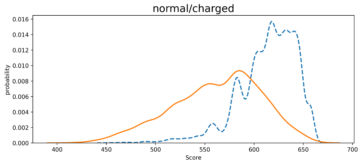
Figure 7. Normal/Default Customer Score Distribution (Test Set)

3. Research Result

The model is evaluated using AUC (Area Under Curve) as the main indicator, which can effectively measure the model's ability to distinguish between defaults and non-defaults [15]. A high AUC value indicates the model's superior performance in credit risk prediction, which can help financial institutions to better manage risks. As Figure 8 shows, this study achieved the result as being 0.84.

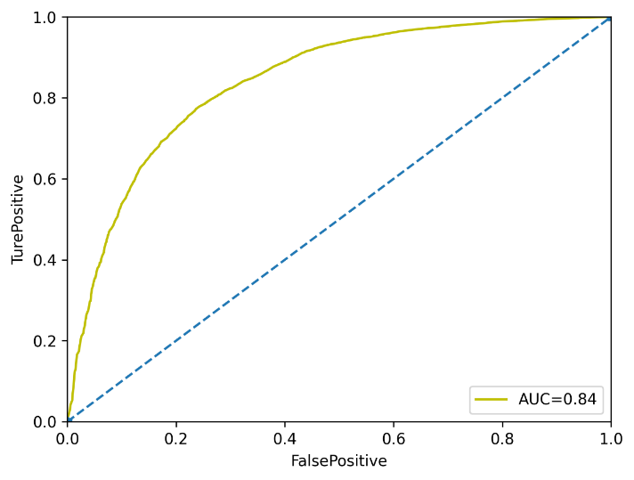
Figure 8. AUC Evaluation

The ROC curve was also plotted to visualize the model’s performance across various threshold values, further confirming the robustness of the logistic regression model.

After training and evaluating the model, it was applied to credit scoring for individual borrowers. For example, one borrower with credit data shown in Table 1 received a score of 613, suggesting they fall in the lower creditworthiness range. This score was derived from their financial history and risk factors as analyzed by the model.

Table 1. Metrics Data from one customer

4. Conclusion

This research emphasizes the importance of the FICO scoring system in contemporary credit assessment, demonstrating how machine learning techniques, including logistic regression, random forest imputation, and feature engineering through Weight of Evidence (WoE) and Information Value (IV), can enhance credit scoring models. By systematically addressing data preprocessing, feature extraction, and model evaluation, this study successfully developed a robust model capable of predicting default risk with a high degree of accuracy, achieving an AUC score of 0.84.

The limitations of the traditional FICO model, particularly its narrow reliance on conventional financial data, were highlighted. As e-commerce, social media, and mobile payments grow in importance, future credit assessment models must incorporate alternative data sources to enhance accuracy and predictive power. The research advocates for integrating these non-traditional data inputs to create more comprehensive credit profiles, ensuring the model better captures modern financial behavior. Alternative models, such as VantageScore, also offer promising directions for future development, complementing FICO's framework.

The role of big data in automating and improving credit evaluation processes is central to this study. By utilizing advanced analytics, financial institutions can reduce biases inherent in manual assessments while increasing efficiency. Nonetheless, the research identifies areas for improvement, particularly the potential for employing more advanced algorithms, such as deep learning, to further enhance model accuracy. Expanding datasets to encompass diverse borrower profiles would also increase fairness and representation.

In conclusion, while FICO remains a widely accepted credit assessment tool, this study suggests that its evolution, through the integration of innovative data sources and machine learning techniques, is necessary to meet the demands of an increasingly digital economy. Enhancing the model's predictive capacity and adaptability will enable more accurate and equitable credit assessments, benefiting both financial institutions and borrowers.

Authors Contribution

All the authors contributed equally and names were listed in alphabetical order.

References

[1]. Mester, L. J. (1997). What’s the point of credit scoring?. Business Review, 3, 3-16.
[2]. Thomas, L. C., Crook, J. N., & Edelman, D. B. (2017). Credit scoring and its applications. SIAM.
[3]. Baesens, B., Van Gestel, T., Stepanova, M., Suykens, J., & Vanthienen, J. (2003). Benchmarking logistic regression and support vector machine classifiers for credit scoring. Journal of the Operational Research Society, 54(6), 627-635.
[4]. Lessmann, S., Baesens, B., Seow, H. V., & Thomas, L. C. (2015). Benchmarking state-of-the-art classification algorithms for credit scoring: An update of the research literature. European Journal of Operational Research, 247(1), 124-136.
[5]. Bellotti, T., & Crook, J. (2009). Support vector machines for credit scoring and discovery of significant features. Expert Systems with Applications, 36(2), 3302-3308.
[6]. Stekhoven, D. J., & Bühlmann, P. (2012). MissForest—non-parametric missing value imputation for mixed-type data. Bioinformatics, 28(1), 112-118.
[7]. Siddiqi, N. (2012). Credit risk scorecards: Developing and implementing intelligent credit scoring. John Wiley & Sons.
[8]. Fawcett, T. (2006). An introduction to ROC analysis. Pattern Recognition Letters, 27(8), 861-874.
[9]. Hand, D. J. (2009). Measuring classifier performance: a coherent alternative to the area under the ROC curve. Machine Learning, 77(1), 103-123.
[10]. Kshetri, N. (2016). Big data’s role in expanding access to financial services in China. International Journal of Information Management, 36(3), 297-308.
[11]. Baesens, B., Van Gestel, T., Stepanova, M., Suykens, J., & Vanthienen, J. (2003). Benchmarking logistic regression and support vector machine classifiers for credit scoring. Journal of the Operational Research Society, 54(6), 627-635.
[12]. Lessmann, S., Baesens, B., Seow, H. V., & Thomas, L. C. (2015). Benchmarking state-of-the-art classification algorithms for credit scoring: An update of the research literature. European Journal of Operational Research, 247(1), 124-136.
[13]. Stekhoven, D. J., & Bühlmann, P. (2012). MissForest—non-parametric missing value imputation for mixed-type data. Bioinformatics, 28(1), 112-118.
[14]. Siddiqi, N. (2012). Credit risk scorecards: Developing and implementing intelligent credit scoring. John Wiley & Sons.
[15]. Fawcett, T. (2006). An introduction to ROC analysis. Pattern Recognition Letters, 27(8), 861-874.
Cite this article
Li,Y.;Shi,Y. (2024). Credit Evaluation System Based on FICO. Applied and Computational Engineering,96,48-55.
Data availability
The datasets used and/or analyzed during the current study will be available from the authors upon reasonable request.
Disclaimer/Publisher's Note
The statements, opinions and data contained in all publications are solely those of the individual author(s) and contributor(s) and not of EWA Publishing and/or the editor(s). EWA Publishing and/or the editor(s) disclaim responsibility for any injury to people or property resulting from any ideas, methods, instructions or products referred to in the content.
About volume
Volume title: Proceedings of the 2nd International Conference on Machine Learning and Automation
© 2024 by the author(s). Licensee EWA Publishing, Oxford, UK. This article is an open access article distributed under the terms and
conditions of the Creative Commons Attribution (CC BY) license. Authors who
publish this series agree to the following terms:
1. Authors retain copyright and grant the series right of first publication with the work simultaneously licensed under a Creative Commons
Attribution License that allows others to share the work with an acknowledgment of the work's authorship and initial publication in this
series.
2. Authors are able to enter into separate, additional contractual arrangements for the non-exclusive distribution of the series's published
version of the work (e.g., post it to an institutional repository or publish it in a book), with an acknowledgment of its initial
publication in this series.
3. Authors are permitted and encouraged to post their work online (e.g., in institutional repositories or on their website) prior to and
during the submission process, as it can lead to productive exchanges, as well as earlier and greater citation of published work (See
Open access policy for details).