1. Introduction

With the widespread application of the Internet of Things (IoT) technology in agriculture, smart farming has gradually become an important means to improve agricultural productivity. IoT technology allows farmers and agricultural researchers to obtain a vast amount of real-time data about the environment and crop growth. These data not only include traditional agricultural information (such as the average number of plant leaves and average root length) but also more detailed sensor data (such as the percentage of vegetative growth dry matter, the average chlorophyll content in plants, and the percentage of root growth dry matter) [1]. This provides unprecedented opportunities for precise management and optimization of agricultural production. However, despite the ease of acquiring data, extracting valuable insights from this large-scale, multidimensional data to optimize agricultural production remains a significant challenge. The complexity of the data, its non-linearity, and the interactions between multiple variables require advanced data analysis tools to achieve effective decision support [2].

In recent years, the application of machine learning technology in agriculture has gained widespread attention. By utilizing machine learning models, particularly regression and classification algorithms, researchers can build predictive models from vast amounts of IoT data. These models can be used to predict crop yields, risks of pest infestations, and environmental stressors (such as frost) [3]. Such models enable farmers to make more informed decisions, thereby increasing agricultural yields and reducing resource wastage. However, despite their excellent performance in terms of prediction accuracy, machine learning models are often seen as “black boxes,” making it difficult for users to understand their internal workings—that is, they cannot clearly identify which input variables have the most significant impact on the model’s output. Therefore, improving the interpretability of machine learning models has become one of the urgent issues in the process of agricultural intelligence [4].

To address this issue, several interpretable machine learning tools have emerged in recent years, such as LIME (Local Interpretable Model-agnostic Explanations). LIME is a model-agnostic explanation tool that explains the predictions of complex machine learning models by constructing locally linear models. This tool can generate explanations for each prediction, helping users understand the contribution of features to the model’s predictions [5]. In the agricultural context, the application of LIME is particularly important because farmers and agricultural experts not only need accurate predictions but also need to understand which variables have the most influence on these predictions. This interpretative analysis can help farmers adjust their farming strategies, such as modifying irrigation plans based on changes in soil moisture or temperature, or taking preventive measures based on climate prediction data to avoid the spread of pests and diseases [6].

This study aims to analyze key factors in an IoT-driven agricultural dataset using regression and classification machine learning algorithms, exploring how the LIME tool can be used to explain feature importance in the models. Specifically, we will use regression models to predict the thirteenth column: percentage of root growth dry matter (PDMRG), and classification models to predict the fourteenth column: the origin of the crops. By incorporating LIME, we aim to better understand which features play a significant role in the model’s predictions and provide practical optimization suggestions for agricultural production.

The structure of this paper is as follows: Section 2 presents a literature review, summarizing the application of IoT technology in agriculture, the achievements of regression and classification models in agricultural prediction, and the progress in research on interpretability tools such as LIME. Section 3 introduces our research methodology, including a description of the dataset, feature engineering, model selection and evaluation metrics, and the specific application of the LIME tool. Section 4 presents the experimental results, compares the performance of different models, and analyzes and discusses the feature importance results generated by LIME. Finally, Section 5 summarizes the key research findings, discusses the limitations of this study, and proposes potential directions for future research.

2. Literature Review

The literature review summarizes existing research, highlights research gaps, and clarifies the innovative contributions of your study.

In recent years, the application of IoT technology and random forest algorithms in agriculture has been increasingly common. Everingham et al. used a random forest algorithm to accurately predict sugarcane yields. Simulated biomass from the APSIM (Agricultural Production Systems Simulator) sugarcane crop model, seasonal climate forecast indices, and observed rainfall, maximum and minimum temperatures, and radiation were provided as inputs to a random forest classifier and random forest regression model to explain the annual variations in sugarcane yield in the Tully region of northeastern Australia [7].

Bovo et al. analyzed random forest models for dairy cattle milk production under heat stress conditions using machine learning algorithms. Their data were effectively used to calibrate numerical models to predict future trends in animal production. On the other hand, machine learning methods in Precision Livestock Farming (PLF) are now regarded as promising solutions in the field of livestock research, with applications in dairy farming improving sustainability and efficiency in the industry. This study aimed to define, train, and test models developed using machine learning techniques, adopting the random forest algorithm, with the primary goal of evaluating the relationship trends between daily milk production per cow and environmental conditions. However, it did not delve into the specific contributions of features to the model [8].

Edeh et al. used boosted random forests and CHAID to predict white spot disease (WSD) in shrimp farms. Given the growing concern over the severity of this disease, the study employed visualization and machine learning algorithms to provide shrimp farmers with a predictive model for diagnosing and detecting WSD. The study utilized a dataset from the Mendeley repository. The machine learning algorithms—random forest classification and CHAID—were employed for the study, with Python used to implement the algorithms and visualize the results. The obtained results showed a high prediction accuracy (98.28%), indicating that the model was suitable for accurate disease prediction. This study enhances awareness of managing white spot disease in shrimp farming using technology and ensures real-time prediction during and after the COVID-19 pandemic [9].

Ayoola et al. employed a data-driven framework for precision agriculture that optimized crop classification using random forest methods, utilizing machine learning algorithms and agricultural data. By analyzing variables such as soil nutrient levels, temperature, humidity, pH, and rainfall, this system provided tailored recommendations for crop selection and planting practices. This approach optimized resource utilization, improved crop productivity, and promoted sustainable agriculture [10].

In comparison, a research gap can be identified in the existing studies: most of them focus solely on the predictive performance of models while neglecting the need to interpret the results. In agricultural production, farmers and decision-makers are more interested in understanding which environmental factors significantly impact yields or crop health. Therefore, research that integrates interpretability tools can provide more practical value for agriculture. This study combines multiple machine learning algorithms and the LIME interpretability tool to conduct a more comprehensive feature analysis of IoT-driven agricultural datasets.

3. Methodology

This section details the key components of the study, including a description of the dataset, the implementation of feature engineering, the model selection process, the definition of evaluation metrics, the choice of algorithms, and the application of the LIME method.

This study utilized an IoT agricultural dataset that encompasses a wide range of data related to crop growth attributes. These data provided a rich information base for analyzing and predicting crop growth.

In terms of model selection, we employed two categories of machine learning algorithms. First, regression algorithms (such as linear regression and random forest regression) were used to predict the percentage of dry matter in root growth (PDMRG). These algorithms effectively capture the relationships between continuous variables and provide in-depth analysis of root growth. Second, classification algorithms (such as logistic regression and support vector machines) were employed to predict crop growth regions. These algorithms are suitable for handling classification problems and assist in identifying the distribution of crops under different environmental conditions.

To enhance model interpretability, this study also employed the LIME to analyze the importance of features in-depth. Using LIME, we were able to evaluate the specific impact of each feature on the prediction results, revealing the key factors in the model’s decision-making process. This interpretability not only aids in understanding the model’s output but also provides a foundation for subsequent decision-making, allowing agricultural managers to make more precise, data-driven decisions.

3.1. Dataset

The dataset used in this study was part of a master’s thesis conducted by Mohammed Ismail Lifta (2023-2024), a student in the Department of Computer Science at the College of Computer Science and Mathematics, University of Tikrit, Iraq. The research data came from agricultural laboratories and involved plants grown in IoT-enabled greenhouses and traditional greenhouses [11]. The study was supervised by Prof. Wisam Dawood Abdullah (Assistant) of the Cisco Networking Academy/University of Tikrit.

The dataset contains 30,000 entries and 14 columns, providing comprehensive information on various plant indicators related to plant nutrition and root growth, all in floating-point data format, as shown in Table 1: IoT Farming.

Table 1. IoT Farming.

3.2. Model Selection and Evaluation

In this study, both regression and classification models were selected. The regression models include Mean Squared Error regression (MSE regression), while the classification models involve multi-class classification models. The performance of the models was evaluated using several metrics, including R², Mean Squared Error (MSE), Root Mean Squared Error (RMSE), Accuracy, and F1 Score.

3.2.1. R² (Coefficient of Determination)

R² represents the proportion of variance between the independent and dependent variables that the model explains, measuring the goodness of fit.

The formula is:

\( {R^{2}}=1-\frac{\sum _{i=1}^{n}({y_{i}}-{\hat{y}_{i}}{)^{2}}}{\sum _{i=1}^{n}({y_{i}}-\overline{y}{)^{2}}} \)

Where \( {y_{i}} \) is the actual value, \( {y_{i}} \) is the predicted value, \( \overset{\_}{y} \) is the mean of the actual values, and n is the number of samples.

3.2.2. Mean Squared Error (MSE)

MSE measures the difference between the predicted and actual values, with smaller values indicating better performance.

The formula is:

\( MSE=\frac{1}{n}\sum _{i=1}^{n}({y_{i}}-{\hat{y}_{i}}{)^{2}} \)

Where \( {y_{i}} \) is the actual value, \( \hat{{y_{i}}} \) is the predicted value, and n is the number of samples.

3.2.3. Accuracy

In classification models, accuracy measures the proportion of correct predictions.

The formula is:

\( Accuracy=\frac{TP+TN}{TP+TN+FP+FN} \)

Where TP is True Positive, TN is True Negative, FP is False Positive, and FN is False Negative.

3.2.4. F1 Score

The F1 Score is the harmonic mean of Precision and Recall, mainly used for imbalanced datasets.

The formula is:

\( F1=2×\frac{Pr{e}cision×Re{c}all}{Pr{e}cision+Re{c}all} \)

Where:

\( Precision=\frac{TP}{TP+FP},Re{c}all=\frac{TP}{TP+FN} \)

These mathematical formulas help explain the performance of the models and provide a basis for comparison.

3.2.5. RMSE (Root Mean Squared Error)

RMSE is a commonly used evaluation metric for regression models, measuring the difference between predicted and actual values. It is the square root of the MSE, with lower values indicating smaller prediction errors.

The formula is:

\( RMSE=\sqrt[]{\frac{1}{n}\sum _{i=1}^{n}({y_{i}}-{\hat{y}_{i}}{)^{2}}} \)

Where \( {y_{i}} \) is the actual value, \( \hat{{y_{i}}} \) is the predicted value, and n is the number of samples. RMSE intuitively represents the distance between predicted and actual values, making it easier to interpret than MSE.

3.3. Machine Learning Algorithms

The regression models include MSE regression, while the classification models involve multi-class classification models. For regression tasks, the MSE regression model was used, which optimizes the results by minimizing the mean squared error between predicted and actual values. MSE is a commonly used loss function in regression tasks, as it measures the performance of the model by calculating the differences between the predicted and actual values. MSE regression is highly effective for predicting continuous target variables, especially for tasks such as predicting plant growth indicators in agricultural data. Due to its simple calculation and strong statistical properties, MSE regression performs well in many applications.

For classification tasks, multi-class classification models were employed to predict discrete class labels. Common multi-class classification models include Logistic Regression, Support Vector Machines (SVM), and Random Forest classifiers. These models learn the differences between categories within the data to classify unseen data. Multi-class classification models are particularly well-suited for tasks like crop origin prediction, where the goal is to assign plants to different categories based on input features. In classification models, the objective is to improve model performance by maximizing metrics like Accuracy and F1 Score.

3.4. Interpretability Analysis

In the interpretability analysis section of this paper, to visually display the prediction results of the regression and classification models, we utilized the LIME. LIME is a general explanation tool that generates local linear models, revealing how different features influence prediction results and helping us understand the decision-making process of complex machine learning models.

In the interpretability analysis of the classification model, LIME generates a ranking of feature importance based on the model’s prediction results, showing which features played a major role in the classification outcome. The explanations produced by LIME provide clear visual charts for each prediction, illustrating the positive or negative impact of each feature.

In the interpretability analysis of the regression model, LIME reveals the contribution of each feature to the predicted value, helping us identify which factors had the greatest influence on the prediction results. This interpretability analysis not only improves model transparency but also offers agricultural managers practical guidance, aiding in the optimization of agricultural production strategies.

4. Experimental Results

4.1. Performance of Regression and Classification Models

As shown in Table 2, after fine-tuning the XGBOOST parameters—maximum tree depth, learning rate, and root mean squared error—the R² of the Mean Squared Error regression model was 1, the MSE was 0.01, and the RMSE was 0.12. This indicates that the linear regression model performed excellently in predicting the percentage of root growth dry matter (PDMRG). In the Random Forest classification model, ten sets of screened data were used to predict the plant origin regions, and the F1, Accuracy, and Precision scores were all 1, indicating that all regions were predicted with complete accuracy.

4.2. Visualization of Regression and Classification Data

The Figure 1 demonstrates the trade-off between the True Positive Rate (TPR) and the False Positive Rate (FPR) in the classification model. For each class, the model generates a series of TPR and FPR values by adjusting the classification threshold. Generally, as TPR increases, FPR also rises. The ROC curve reflects the performance variation under different thresholds.

The horizontal axis (X-axis) represents the False Positive Rate, which is the proportion of negatives incorrectly classified as positives (false positive rate).

The vertical axis (Y-axis) represents the True Positive Rate, which is the proportion of positives correctly classified as positives (true positive rate).

The black dashed line indicates the performance of a random classifier, where TPR equals FPR, serving as a benchmark. If the classifier performs better than random guessing, the curve will deviate from this line.

An AUC (Area Under the Curve) of 1.00 indicates the classifier perfectly distinguishes between positive and negative classes. In this figure, the AUC for all six classes is 1.00, signifying flawless prediction performance, with no classification errors. This means that the TPR for each class reaches 100%, while the FPR is 0%.

The ROC curve illustrates that the model’s classification performance for these six classes is perfect (AUC = 1.00), showcasing its strong ability to distinguish between categories in the test data.

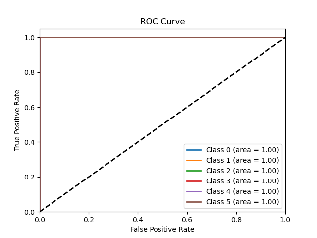
Figure 1. ROC Curve

As shown in Figure 2, the X-axis (Actual Values) represents the actual values in the dataset, i.e., the true values of the target variable in the training or testing set. The Y-axis (Predicted Values) represents the predicted values from the regression model, which are the outputs the model generates based on the input features. Each blue dot on the scatter plot represents the relationship between an actual value and its corresponding predicted value. The black dashed line is the reference line, indicating the ideal situation where the predicted values equal the actual values. If all data points lie on this line, it indicates the model’s predictions perfectly match reality, reflecting excellent performance.

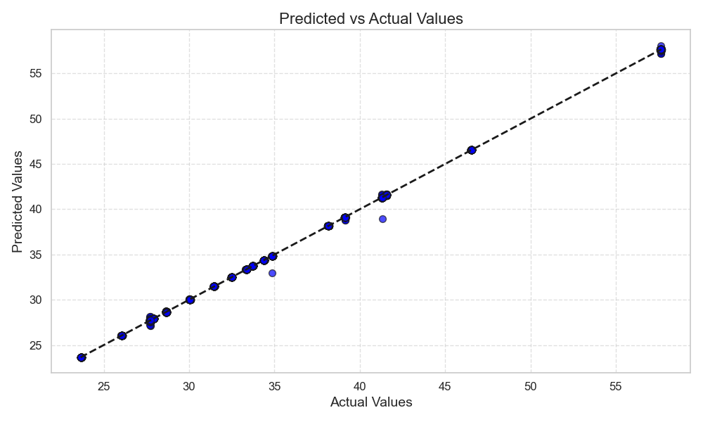
Figure 2. Predicted vs Actual Values.

4.3. Feature Importance Analysiss

Through LIME analysis, we identified ARD, PHR, and PDMVG as the three most important features for predicting crop origin. Among them, ARD had the highest contribution to the linear regression model’s predictions, while PDMVG exhibited strong interpretability in the classification algorithm, and PHR and AWWR had higher interpretability in the random forest model.

As shown in Figure 3, the classification algorithm uses the LIME interpreter. The LIME-generated chart displays the top 10 features from the dataset that have the greatest impact on predicting crop origin. The length of the bars represents the degree of influence each feature has on the prediction. The longer the bar, the greater the feature’s influence on the prediction outcome. The horizontal axis represents the contribution value of each feature to the model’s prediction. The larger the contribution value, the greater the feature’s impact on the final classification result. Positive contributions are shown in green, indicating that an increase in the feature value helps predict Class 1, while negative contributions are shown in red, indicating that an increase in the feature value suppresses the prediction of Class 1. The contribution values range from -0.15 to 0.025, representing the relative influence of each feature on the classification decision.

The vertical axis lists the top 10 important features affecting the model’s predictions, with the value range of each feature labeled next to it. These features include:

PHR: When the value is less than or equal to 51.06, it has a strong negative impact on predicting Class 1 (indicated in red).

PDMVG: When PDMVG is greater than 27.71, it has a positive effect on predicting Class 1 (indicated in green).

ALAP and ADWV show varying degrees of positive and negative contributions to the prediction outcome.

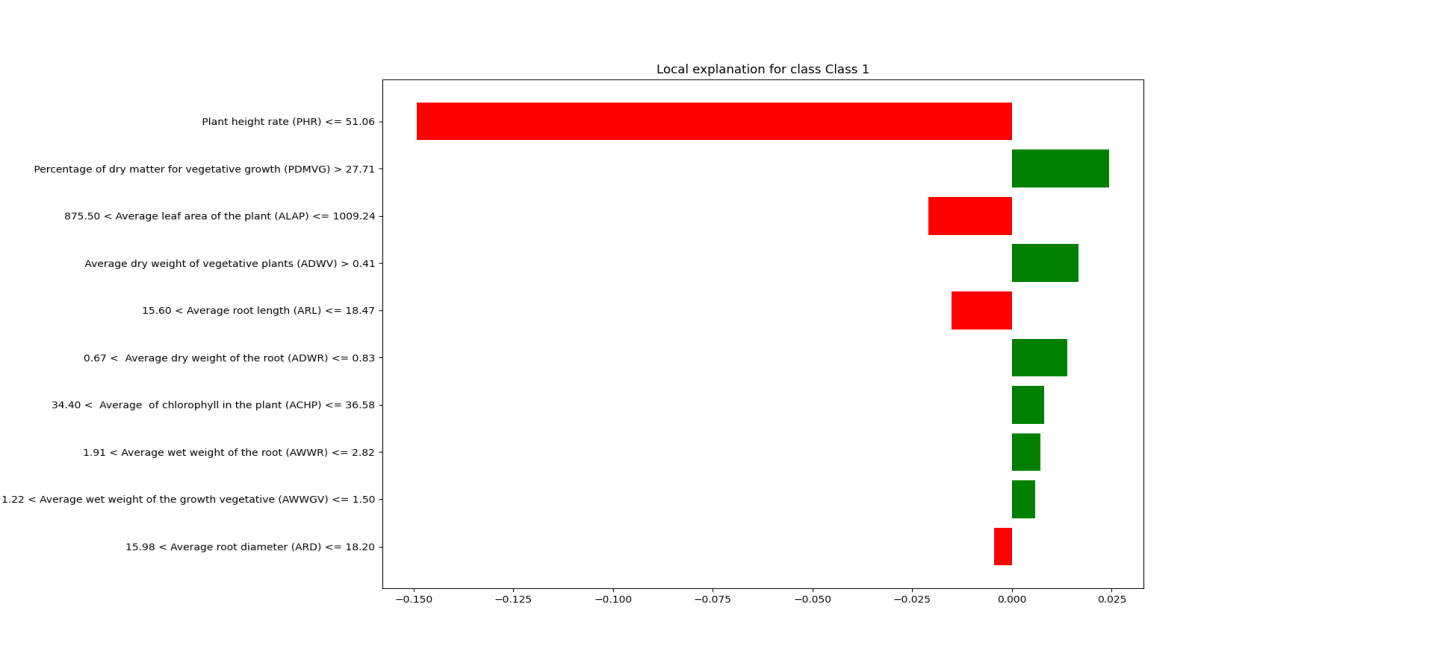
Figure 3. Classification Prediction

The legend indicates that the most influential factors in helping the classification algorithm predict crop origin, ranked from highest to lowest, are PDMVG, ADWV, ADWR, ACHP, AWWR, and AWWGV. This suggests that in agricultural trade, farmers can monitor these plant data points to make more informed decisions about crop origin.

The horizontal axis represents the impact of features on the predicted value, with a range from -2.0 to 1.0. Values closer to 0 indicate a smaller effect on the prediction, while larger values indicate stronger positive contributions, and smaller values indicate stronger negative impacts,, as shown in Figure 4. Positive contributions are represented by green bars, showing that an increase in the feature value raises the predicted value. Negative contributions are represented by red bars, showing that an increase in the feature value lowers the predicted value.

The vertical axis lists the top 10 most important features in the model, along with their value ranges. LIME explains how the specific values of these features affect the prediction result at this particular data point. Each row represents the range of a feature value that has the most significant impact on the prediction outcome. For example:

ANPL: When the feature value is between 3.01 and 4.00, it has the largest negative impact on the prediction result (indicated in red, with a contribution value of about -2.0).

ADWR: When the feature value is between 0.68 and 0.83, it also has a significant negative impact on the prediction result (with a contribution value of about -1.0).

The features with the largest negative contributions are the ANPL and the ADWR, as their feature values within certain ranges lead to a decrease in the model’s predicted values. The features with the largest positive contributions are PHR and AWWR, suggesting that higher values for these features lead to an increase in predicted values.

The legend indicates that the most beneficial factors for regression algorithm prediction, ranked from highest to lowest, are PHR, AWWR, and ALAP. This suggests that in agricultural production, farmers can monitor these three values to achieve higher PDMRG scores, which equates to healthier crop root systems.

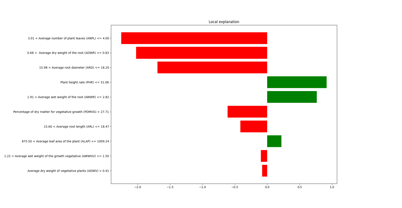
Figure 4. Regression Prediction

5. Discussion

The experimental results indicate that the random forest regression model excels at handling nonlinear data. Furthermore, the LIME explanation results reveal the significant impact of crop PDMRG values on root health, which aligns with existing agricultural theories. However, the varying importance of certain features across different models in this study may reflect the different ways each model processes data patterns.

In this study, through the regression and classification model analysis of IoT agricultural datasets, we identified the impact of key features on the prediction targets, such as the PDMRG and crop origin. The random forest regression model performed exceptionally well in managing nonlinear data, particularly after feature selection and data preprocessing, resulting in a significant increase in predictive accuracy, consistent with findings in the existing literature. According to the LIME explanation results, the model was able to identify the features that had the most substantial impact on yield predictions, including the ARL and the AWWR. These features hold considerable practical significance in agricultural production, as they directly influence a plant’s ability to absorb moisture and nutrients from the soil.

In the classification task, LIME revealed the significant role of features such as the ACHP and the ALAP in predicting crop origin. This indicates that environmental factors have a profound impact on crop growth performance, aligning with the widely recognized theoretical foundations in the agricultural field.

However, it is noteworthy that the importance of certain features varies across different models. For instance, in the regression model, ARD has a high predictive contribution, while its influence in the classification model is comparatively small. This discrepancy may reflect the different ways each model processes feature patterns and could also be related to noise and biases present in agricultural data.

6. Conclusion

This study compared the application effectiveness of regression and classification models in agricultural predictions using IoT agricultural datasets and introduced the LIME explanation tool to enhance model interpretability. The results show that both linear regression and random forest regression performed well in predicting the percentage of dry matter in root growth, while logistic regression and support vector machines excelled in predicting crop origin. Additionally, the LIME interpreter provided intuitive explanations for the feature contributions of each model, helping users understand which variables had the most significant impact on prediction outcomes.

Despite the promising results, this study also has some limitations. For example, the dataset did not consider temporal factors; future research could incorporate time series analysis techniques to explore the impact of environmental variables on crop predictions at different time points. Furthermore, additional external environmental factors, such as weather forecast data, could be introduced to further optimize the predictive capabilities of the models.

Future research directions may focus on multi-model ensemble techniques, integrating emerging algorithms such as deep learning and reinforcement learning to enhance the accuracy and practicality of models, thereby driving the innovative development of smart agricultural systems.

References

[1]. R. Akhter and S. A. Sofi, “Precision agriculture using IoT data analytics and machine learning,” Journal of King Saud University-Computer and Information Sciences, vol. 34, no. 8, pp. 5602-5618, 2022.
[2]. K. S. P. Reddy, Y. M. Roopa, K. R. LN, and N. S. Nandan, “IoT based smart agriculture using machine learning,” in 2020 Second international conference on inventive research in computing applications (ICIRCA), 2020: IEEE, pp. 130-134.
[3]. A. Chlingaryan, S. Sukkarieh, and B. Whelan, “Machine learning approaches for crop yield prediction and nitrogen status estimation in precision agriculture: A review,” Computers and electronics in agriculture, vol. 151, pp. 61-69, 2018.
[4]. R. Zhao, Z. Yang, D. Liang, and F. Xue, “Automated Machine Learning in the smart construction era: Significance and accessibility for industrial classification and regression tasks,” arXiv preprint arXiv:2308.01517, 2023.
[5]. J. Waring, C. Lindvall, and R. Umeton, “Automated machine learning: Review of the state-of-the-art and opportunities for healthcare,” Artificial intelligence in medicine, vol. 104, p. 101822, 2020.
[6]. A. Sharma, A. Jain, P. Gupta, and V. Chowdary, “Machine learning applications for precision agriculture: A comprehensive review,” IEEE Access, vol. 9, pp. 4843-4873, 2020.
[7]. Y. Everingham, J. Sexton, D. Skocaj, and G. Inman-Bamber, “Accurate prediction of sugarcane yield using a random forest algorithm,” Agronomy for sustainable development, vol. 36, pp. 1-9, 2016.
[8]. M. Bovo, M. Agrusti, S. Benni, D. Torreggiani, and P. Tassinari, “Random forest modelling of milk yield of dairy cows under heat stress conditions,” Animals, vol. 11, no. 5, p. 1305, 2021.
[9]. M. O. Edeh et al., “Bootstrapping random forest and CHAID for prediction of white spot disease among shrimp farmers,” Scientific Reports, vol. 12, no. 1, p. 20876, 2022.
[10]. A. J. Ayoola, J. Essien, M. Ogharandukun, and F. Uloko, “Data-Driven Framework for Crop Categorization using Random Forest-Based Approach for Precision Farming Optimization,” European Journal of Computer Science and Information Technology, vol. 12, no. 3, pp. 15-25, 2024.
[11]. W. ABDULLA. “Advanced IoT Agriculture 2024.” https://www.kaggle.com/datasets/wisam1985/advanced-iot-agriculture-2024 (accessed.
Cite this article
Zhang,Z. (2024). Predictive Modeling in IoT-Driven Agriculture: A Comparative Study of Regression and Classification with LIME Interpretability. Applied and Computational Engineering,96,31-41.
Data availability
The datasets used and/or analyzed during the current study will be available from the authors upon reasonable request.
Disclaimer/Publisher's Note
The statements, opinions and data contained in all publications are solely those of the individual author(s) and contributor(s) and not of EWA Publishing and/or the editor(s). EWA Publishing and/or the editor(s) disclaim responsibility for any injury to people or property resulting from any ideas, methods, instructions or products referred to in the content.
About volume
Volume title: Proceedings of the 2nd International Conference on Machine Learning and Automation
© 2024 by the author(s). Licensee EWA Publishing, Oxford, UK. This article is an open access article distributed under the terms and
conditions of the Creative Commons Attribution (CC BY) license. Authors who
publish this series agree to the following terms:
1. Authors retain copyright and grant the series right of first publication with the work simultaneously licensed under a Creative Commons
Attribution License that allows others to share the work with an acknowledgment of the work's authorship and initial publication in this
series.
2. Authors are able to enter into separate, additional contractual arrangements for the non-exclusive distribution of the series's published
version of the work (e.g., post it to an institutional repository or publish it in a book), with an acknowledgment of its initial
publication in this series.
3. Authors are permitted and encouraged to post their work online (e.g., in institutional repositories or on their website) prior to and
during the submission process, as it can lead to productive exchanges, as well as earlier and greater citation of published work (See
Open access policy for details).