1. Introduction

In the contemporary landscape of signal processing, the challenge of effectively denoising and predicting signal waveforms stands as a critical focal point for researchers and practitioners alike. Liu and Xu’s research on the WTMM algorithm [1] and Dragoman, D’s research on Wigner distribution function [2] are great examples of problem-solving. Signal waves, which are omnipresent in various applications such as telecommunications, biomedical engineering, and environmental monitoring, often suffer from noise and interference. These extraneous components can significantly hinder the accuracy and reliability of the signal analysis, thereby necessitating the development of effective denoising and prediction methods. Unlike traditional complex denoising and prediction methods, this paper aims to explore the feasibility of using machine learning to process signals. It can to some extent solve the problem of signal denoising and prediction being too cumbersome in specific situations, and also proposes a new approach. This paper delves into the realm of signal denoising and prediction, specifically through the lens of regression models. Regression models, renowned for their simplicity and interpretability, offer a potent tool for modelling and mitigating noise within signals. The primary objective of this research is to explore and evaluate the efficacy of various regression-based techniques in the context of three distinct types of signal waves: sinusoidal, linear, and polynomial. Each of these signal types presents unique characteristics and challenges, providing a comprehensive landscape for assessing the performance of the proposed methods. This paper summarizes the relevant theoretical basis by reviewing literature. This article will also compare it with the denoising methods of regression models to explore their advantages and disadvantages. By applying these models to the denoising and prediction tasks, the research aims to quantify their effectiveness through a series of empirical evaluations. The findings of this research are anticipated to contribute significantly to the field of signal processing by highlighting the strengths and limitations of regression models in denoising and predicting diverse signal types. Moreover, this study seeks to lay the groundwork for future advancements in regression-based signal processing techniques, fostering improved accuracy and efficiency in practical applications. Through rigorous analysis and experimentation, this paper aspires to provide valuable insights and practical guidelines for enhancing signal integrity and predictive performance in various technological domains.

2. Features of These Three Signal Waves

2.1. Sinusoidal signal

A sin signal wave is a signal with the most singular frequency component, and its waveform follows the mathematical sin curve, hence its name. A sin signal can be represented as x (t)=Asin (ω*t+φ)=A cos (ω*t+φ-π/2). In the formula, A is the amplitude, ω is the angular frequency (radians/second), and φ is the initial phase angle (radians). Sin signal waves have obvious periodicity characteristics, that is, the same waveform will repeatedly appear within a certain period of time, and the relationship between their period T and frequency function is T=1/f. ‌ A sin wave is a continuous function that exists at any point in time and it also has smooth curve characteristics, without abrupt changes or jumps. ‌Sinusoidal signal waves have become important research objects in fields such as signal and system, circuit theory, etc. due to their unique characteristics and wide applications. They have a wide range of applications in communication, electronics, sound, and other fields.

2.2. Linear signal

A linear signal refers to one whose amplitude changes linearly over time. Mathematically, a linear signal can be represented as: x(t)=a ⋅ t +b. Among them, a and b are constants, and t is a time variable. It has four features as follows. The expression of linear signals is simple and easy to understand and process. It does not have periodic, oscillatory, or complex spectral characteristics. And the rate of change of the signal is determined by the slope a. If a is positive, the signal increases over time; If a is negative, the signal decreases over time. The third point is that a linear expression can accurately predict the future value of the signal, as it changes at a constant rate over time. Finally, the frequency spectrum of a linear signal in the frequency domain is simple and usually concentrated in the low-frequency part because it does not have periodic variations. Linear signals are widely used in various scientific and engineering fields, especially in areas such as system analysis, control systems, and signal processing.

2.3. Polynomial signal

Polynomial signal waves refer to signal waveforms that do not satisfy a linear relationship between the output and input of a signal. This paper uses a quadratic polynomial as an example, as there is no clear formula for polynomial signals. This model has the advantages of being able to handle a variety of image trajectory types and flexible forms, and can dynamically adjust algorithms to prevent overfitting and underfitting [3]. The waveform of Polynomial signals cannot be described by simple mathematical functions, and their behavior is complex and difficult to predict long-term development trends. ‌And some nonlinear signals exhibit similar structures at different scales, known as fractality. Besides that,‌ the signal may undergo drastic changes in a short period of time, and these mutation points often correspond to specific events or state changes. ‌Having chaos is also possible. Polynomial signals may exhibit sensitivity to initial conditions, and small changes can lead to significant changes in the long-term behavior of the signal. ‌Polynomial signal waves have wide applications and research value in various fields such as communication, biomedicine, and geophysics. ‌‌

3. Linear and Polynomial Regression

3.1. Simple introduction

By fitting a linear equation to the observed data, linear regression is a statistical method that models the relationship between a dependent variable and one or more independent variables. Linear regression assumes a linear relationship between independent and dependent variables. It's simple and, easy to interpret and implement, making it one of the most commonly used models in statistics and machine learning. Additionally, it's computationally efficient, particularly for large datasets. However, it has limitations, as it's not suitable for modeling nonlinear relationships unless the data is transformed. Linear regression is widely applied in fields like economics, engineering, and social sciences for prediction, trend analysis, and understanding variable relationships. Just like Jessica Kasza, and Rory Wolfe applied the model to the medical field [4]. Polynomial regression extends linear regression by modeling the relationship between variables as an nth-degree polynomial. It can capture complex, nonlinear relationships by fitting a polynomial curve to the data. While it offers flexibility by allowing higher-degree polynomials to fit more intricate data patterns, this can also lead to overfitting. Additionally, as the degree increases, the model becomes harder to interpret due to the growing complexity of terms. Many types of data are best analyzed by fitting a curve using nonlinear regression, and computer programs that perform these calculations are readily available [5]. Polynomial regression is commonly applied in scenarios where relationships between variables are nonlinear but can be approximated by a polynomial, such as modelling growth rates, temperature variations, and other complex physical phenomena.

3.2. Reasons for using them

Machine learning can be applied to various areas, especially to complex problems that have no clear computational rule or solution [6]. Regression models' fundamental strengths in capturing underlying patterns within data motivate their use for signal denoising and prediction. When dealing with signals—whether they are simple, like sin or linear signals, or more complex, like polynomial signals—noise is an inevitable aspect that can obscure the true signal. The ability of regression models to identify and represent the relationship between the input variables (such as time) and the output (signal values) makes them powerful tools for mitigating the impact of noise. Regression models are effective at recognizing patterns in data, particularly for periodic, linear, or polynomial signals. For example, linear regression can approximate the relationship between time and a noisy sin wave, filtering out noise by fitting the best line or curve to represent the signal's trend. Polynomial regression captures nonlinear relationships, making these models flexible enough to fit various signal types, including complex ones. Beyond denoising, regression models offer predictive power, enabling future signal value predictions based on learned relationships, which is especially useful in fields like communications, finance, and engineering. Their simplicity and interpretability make them preferable over more complex models, while they are robust to certain types of noise by capturing the main signal trend. Furthermore, regression models integrate easily with other signal processing techniques, such as Fourier transforms, enhancing overall performance in signal denoising and prediction.

4. Research Methods and Results

4.1. Using Linear Regression

4.1.1. Methods

The steps of Signal using linear regression for signal denoising are as follows. Step 1 is generating a noisy signal: creating a synthetic signal (e.g., a sine wave or a linear signal) and adding random noise to simulate a noisy signal. Step 2 is fitting linear regression: using the noisy signal as the dependent variable and time as the independent variable. Fit a linear regression model to this data. Step 3 is predicting the denoised signal: using the fitted model to predict the signal values, which should ideally represent the underlying trend, thereby reducing the impact of noise. And the model tries to minimize the difference between the predicted signal values and the noisy signal by adjusting the slope and intercept of the line. This process effectively smooths out the high-frequency noise that does not align with the general trend of the data. The fitted model predicts the signal values at each point in time. Since linear regression fits a straight line, the resulting signal is a smoothed version of the original noisy signal, capturing the general trend and ignoring random fluctuations. The steps of Signal using linear regression for signal prediction are also as follows. Step 1 involves extending the independent variable, specifically the time variable, into the future for prediction purposes. Step 2 is predicting future signal Values: Appling the fitted linear regression model to the extended time variable to predict future signal values. And to predict future signal values, we extend the time variable beyond the range used for training. The model then applies the learned linear relationship to these new time points to generate predictions. The model assumes that the linear relationship between time and signals observed in the past continues into the future. Thus, the predicted signal follows the same slope and intercept, providing a forecast that aligns with the historical trend.

4.1.2. Results and discussion

The picture below shows the results of denoising and predicting different signals using a linear regression model:

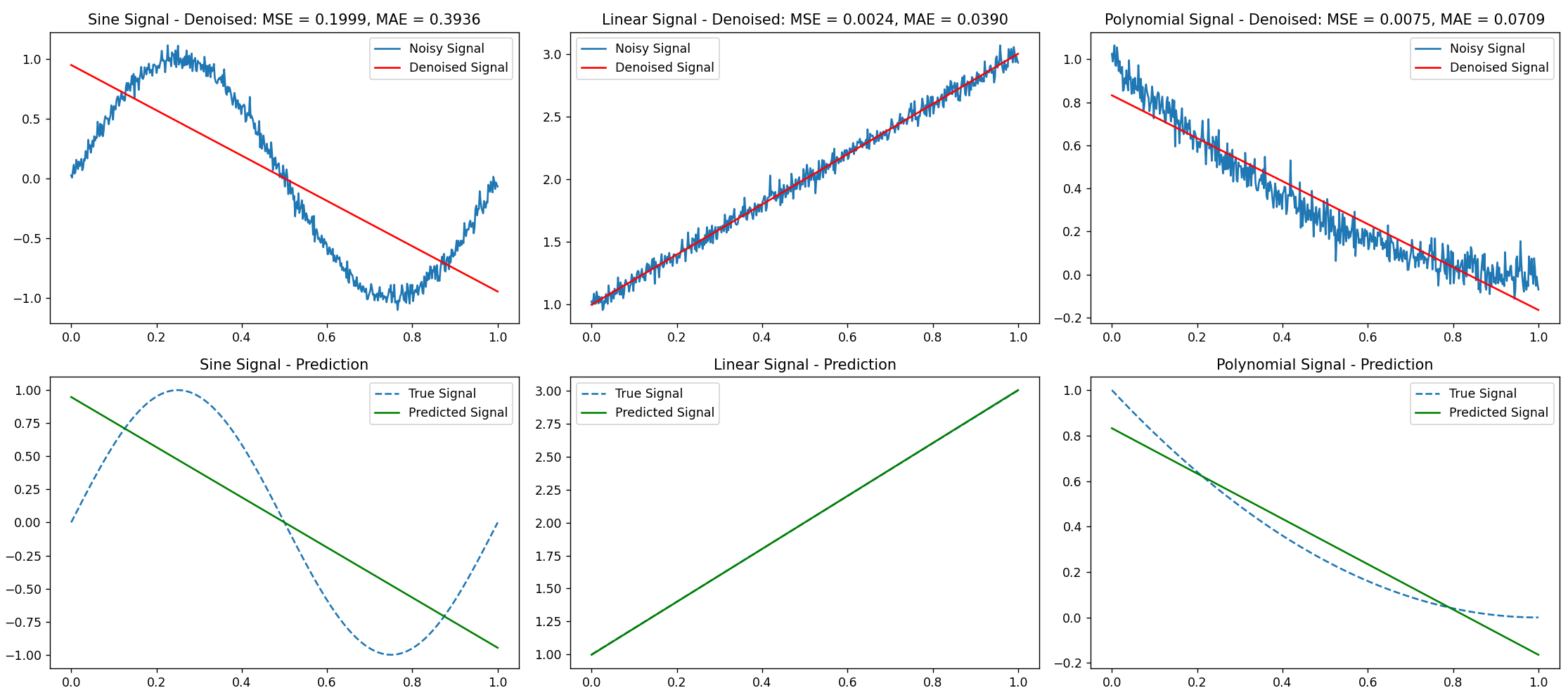
Figure 1. Processing results of linear regression model

Linear regression performed well in denoising the linear signal, accurately fitting the data and effectively smoothing out noise. The denoised signal closely followed the original, with minimal error indicated by low MSE and MAE values. However, linear regression struggled with non-linear signals, such as the sine wave, where it attempted to fit a straight line to periodic data, resulting in poor denoising. The model was unable to capture the oscillatory nature of the sine wave, leading to significant errors and demonstrating the limitation of linear regression with non-linear signals. The polynomial signal posed a similar challenge, as the model’s straight-line approximation could not capture the non-linear trend, resulting in a denoised signal that deviated significantly from the original. In terms of prediction, linear regression successfully extended the linear trend of a linear signal into the future, providing reliable predictions with low error rates. But the model couldn't predict the sine and polynomial signals correctly because it couldn't understand their nonlinear patterns. Linear regression offers simplicity, efficiency, and interpretability, making it easy to implement and interpret for signal denoising and prediction, with model parameters like slope and intercept directly providing insights into the trend. However, its limitations include being restricted to linear trends, making it less effective for signals with non-linear or complex patterns. The model is also sensitive to outliers, which can significantly affect performance by impacting slope and intercept values. Additionally, while linear regression can smooth random noise, it may struggle with high-frequency or systematic noise, limiting its effectiveness in more complex denoising tasks.

4.2. Using Polynomial Regression

4.2.1. Methods

The steps of Signal using polynomial regression for signal denoising are as follows. Step 1 is choosing the polynomial degree: the first step is to determine the appropriate degree for the polynomial. The degree should be high enough to capture the signal's underlying pattern but not so large that it starts fitting the noise as well. Step 2 is fit the polynomial regression model: once the degree is chosen, the polynomial regression model is fitted to the noisy signal data. This involves finding the coefficients β0, β1…, βn that minimize the difference between the observed signal values and the values predicted by the polynomial. Step 3 is predicting the denoised signal: after fitting the model, it can be used to predict the signal values, which will represent a smoothed version of the noisy signal. The higher the degree, the more closely the model will fit the signal, potentially reducing noise but also risking overfitting.

The steps of Signal using polynomial regression for signal prediction are also as follows. Step 1 involves extending the independent variable, such as time, beyond the training model's range for prediction. Step 2 is predicting future signal values: use the fitted polynomial regression model to predict future values of the signal. The model will apply the learned polynomial relationship to the extended time variable, generating predictions based on the captured trend.

4.2.2. Results and discussion

The picture below shows the results of denoising and predicting different signals using a polynomial regression model:

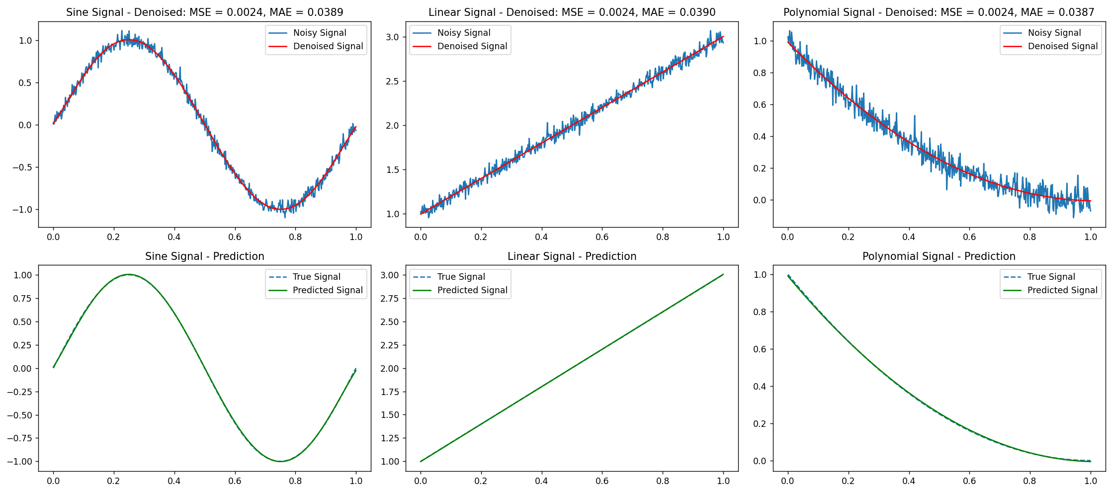
Figure 2. Processing results of Polynomial regression model

Polynomial regression with a degree of 2 or higher did not significantly enhance denoising performance for a linear signal. While it produced a reasonable fit, the model tended to slightly overfit by capturing some noise as part of the signal, resulting in a higher Mean Squared Error (MSE) compared to linear regression, though still achieving acceptable denoising. For the sine signal, polynomial regression notably improved denoising performance relative to linear regression. By using a higher degree polynomial, the model approximated the oscillatory nature of the sine wave, creating a denoised signal closely aligned with the original. However, if the polynomial degree was too high, the model overfitted, capturing noise alongside the signal and slightly increasing the error. For the polynomial signal, polynomial regression excelled at denoising, as a model of appropriate degree could effectively remove noise while preserving the underlying trend, matching the original signal with minimal error and showcasing its strength with non-linear signals. In terms of prediction performance, polynomial regression provided accurate predictions for the linear signal, though a higher-degree polynomial led to minor overfitting and less precise predictions compared to linear regression. With polynomial regression, predictions for the sine signal got a lot better, especially when the degree of the polynomial was well-chosen. This let the model understand that the sine wave is periodic and make good predictions about the future. However, for long-term extrapolation, overfitting led to unrealistic oscillations. Polynomial regression was particularly effective in predicting future values of the polynomial signal, as the correct degree accurately extended the non-linear trend into the future with low error rates. Polynomial regression has notable advantages, including its ability to capture non-linear relationships, making it suitable for signals that do not follow a linear pattern. By fine-tuning the polynomial degree, one can adjust its flexibility to balance signal capture and overfitting. When applied appropriately, it can provide better accuracy in denoising and prediction for non-linear signals compared to linear regression. However, polynomial regression also has limitations, such as the risk of overfitting, where the model captures noise along with the signal, leading to poor generalization to new data. Complexity is another challenge, as increasing the polynomial degree complicates the model and reduces its interpretability, making it less transparent than linear models. Additionally, polynomial regression may yield unreliable predictions when extrapolating far beyond the observed data range, especially at high polynomial degrees.

4.3. Using Fourier Transform(Denoising)

4.3.1. Introduction

The Fourier Transform is a mathematical operation that transforms a signal from the time domain (or spatial domain) into the frequency domain. The main idea is to decompose complex waveforms into a set of simple sinusoidal waves—sin and cos functions. This decomposition makes it easier to analyze the frequency components and characteristics of the signal. The Fourier transform allows us to study the frequency content of a variety of complicated signals. With the explosion of digital data, both in quantity and diversity, the generalization of the tools based on Fourier transform is mandatory [7]. We can view and even manipulate such information in a Fourier or frequency space [8].

Formula:

For a continuous-time signal x(t), the Fourier Transform X(f) is given by:

\( X(f)=\int _{-∞}^{∞}x(t){e^{-j2πft}}dt \)

where f is the frequency and j are the imaginary unit.

For a discrete-time signal x[n], the Discrete Fourier Transform (DFT) is:

\( X[k]=\sum _{n=0}^{N-1}x[n]{e^{-j2πkn/N}} \)

where N is the length of the signal and k is the frequency index.

The above is the transformation formula, and the below is the inverse transformation formula.

Continuous-time signal inverse Fourier Transform:

\( x(t)=\int _{-∞}^{∞}X(f){e^{j2πft}}df \)

Discrete-time signal inverse Fourier Transform:

\( x[n]=\frac{1}{N}\sum _{n=0}^{N-1}X[k]{e^{j2πkn/N}} \)

4.3.2. Methods

Step 1 is applying Fourier transform: the first step in denoising is to apply the Fast Fourier Transform (FFT) to the noisy sin signal. FFT is an efficient algorithm to compute the Discrete Fourier Transform (DFT), which converts the time-domain signal into its frequency components. The result of the FFT is a complex-valued array where each element represents the amplitude and phase of a specific frequency component. Step 2 is analyzing the frequency spectrum: once the signal is transformed into the frequency domain, you can observe the frequency spectrum. The sin wave will manifest as a peak at its fundamental frequency f0. Noise, on the other hand, may appear as lower amplitude components spread across a wide range of frequencies, rather than concentrated at a single frequency. Step 3 is filtering the noise: a common method for denoising involves applying a threshold to the frequency components. Frequencies with amplitudes below a certain threshold are considered noise and are set to zero. Alternatively, this research applies a band-pass filter that isolates the frequencies close to the sin wave's fundamental frequency f0​ and removes other components. This approach preserves the sine wave while eliminating noise that lies outside the band. For targeted noise reduction, this research zero out specific frequency ranges that are identified as noise, while retaining the peak corresponding to the sin wave. Step 4 is applying inverse Fourier transform: after filtering the noise in the frequency domain, the next step is to transform the signal back to the time domain using the Inverse Fast Fourier Transform (IFFT). The IFFT reconstructs the time-domain signal using the modified frequency components, resulting in a denoised version of the original sin wave.

4.3.3. Result and discussion

Here is a picture of the result of using Fourier transform to denoise sin signals:

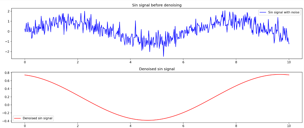
Figure 3. Processing results using Fourier transform

The Fourier transform performed exceptionally well in denoising the sin signal. Since the sin wave is inherently periodic and represented by a single frequency in the frequency domain, the transform could easily separate the signal from the noise, resulting in a clean, denoised output.

The Fourier Transform is highly effective in removing noise from a signal, particularly when the noise is high-frequency and the signal of interest is low-frequency, making it efficient for noise separation. It also offers clear frequency analysis by providing an interpretable frequency spectrum, which aids in understanding the signal’s periodic nature and supports future value predictions. The Fourier Transform’s versatility enables it to handle various types of signals, including both periodic and quasi-periodic signals, making it a widely used tool in signal processing. However, it has limitations, particularly with non-stationary signals, where frequency components change over time. In these cases, the Fourier Transform may be less effective, and alternatives like the Wavelet Transform might be better suited. Another drawback is its loss of time information; while it provides excellent frequency resolution, it lacks time information, making it challenging to analyse transient signals where the timing of frequency changes is critical.

5. Conclusion

Through experiments and comparisons, this paper successfully proves that machine learning models can be used in the computer field to process signal waves. This opens up a new way to study simpler signal processing methods. The specific advantages and disadvantages, as well as possible improvement measures, are as follows. Linear regression is a straightforward method for signal denoising and prediction, particularly effective for signals with a clear linear trend. Its simplicity, efficiency, and interpretability make it a useful baseline in signal processing, ideal for denoising signals with linear relationships and offering quick calculations, though it has limitations for more complex signals. Polynomial regression provides greater flexibility, especially for non-linear signals, as it can smooth noise and give accurate predictions if the polynomial degree is chosen carefully to avoid overfitting. However, its application demands attention to model complexity and extrapolation risks. Fourier Transform excels at denoising periodic signals, effectively removing high-frequency noise and outperforming regression models in this context. While it cannot directly predict signals and requires complex computations and threshold selection, it is highly suitable for denoising periodic signals. While this study demonstrates the effectiveness of linear and polynomial regression models for signal denoising and prediction, comparing them with the Fourier Transform, there are several potential research directions to explore further. First, future research could investigate processing more complex signal types, such as mixed signals or those with non-periodic noise, to validate model effectiveness in varied practical applications and enhance generalization. Additionally, other regression methods like ridge regression, LASSO regression, or support vector regression (SVR) could be explored for their denoising and predictive performance. Another promising direction is the application of deep learning; recent advancements in signal processing using deep neural networks, such as convolutional neural networks (CNNs) or recurrent neural networks (RNNs), could be applied for comparison with traditional regression models. Adaptive regression models that dynamically adjust parameters based on signal characteristics may also be beneficial for handling non-stationary signals. Further research could examine high-dimensional data processing, focusing on effectively applying regression methods in high-dimensional spaces and exploring dimensionality reduction techniques. Real-time application and optimization is another critical area, as future research could optimize regression models to achieve real-time signal processing and validate them in practical systems. Lastly, integrating advanced noise models and filtering techniques with regression models could be explored to enhance denoising performance. Exploring these directions could improve signal denoising and prediction accuracy, expand model applicability, and drive technological progress in related fields.

References

[1]. Yi. Liu, Xu. Cheng; “A New Signal Denoising Algorithm from Wavelet Modulus Maxima.” Fourth International Conference on Fuzzy Systems and Knowledge Discovery (FSKD 2007), Haikou, China, 2007, pp. 32-35, doi: 10.1109/FSKD.2007.90.
[2]. Dragoman, D (2005); “Applications of the Wigner distribution function in signal processing Wigner.” Volume 2005, Issue 10, Page1520-1534.
[3]. T. Bakibayev, A. Kulzhanova; “Common Movement Prediction using Polynomial Regression.” 2018 IEEE 12th International Conference on Application of Information and Communication Technologies (AICT), Almaty, Kazakhstan, 2018, pp. 1-4, doi: 10.1109/ICAICT.2018.8747047.
[4]. Jessica Kasza, Rory Wolfe (2014); “Interpretation of commonly used statistical regression models.” RESPIROLOG, Volume 19, Issue 1, Page 14-21.
[5]. Motulsky H J, Ransnas L A (1987); “Fitting curves to data using nonlinear regression: a practical and nonmathematical review.” FASEB journal, Volume 1, Issue 5, Page 365-374.
[6]. H. -I. Lim; "A Linear Regression Approach to Modeling Software Characteristics for Classifying Similar Software." 2019 IEEE 43rd Annual Computer Software and Applications Conference (COMPSAC), Milwaukee, WI, USA, 2019, pp. 942-943, doi: 10.1109/COMPSAC.2019.00152.
[7]. Benjamin Ricaud, Pierre Borgnat, Nicolas Tremblay, Paulo Gonçalves, Pierre Vandergheynst (2019); “Fourier could be a data scientist: From graph Fourier transform to signal processing on graphs.” Comptes Rendus. Physique, Volume 20, no. 5, pp. 474-488.
[8]. Gallagher TA, Nemeth AJ, Hacein-Bey L (2008); “An introduction to the Fourier transform: Relationship to MRI. American Journal of Roentgenology” Volume 190, Issue 5.
Cite this article
Chen,S. (2024). Research on the Signal Denoising and Prediction Methods Based on Regression Models: Taking Three Types of Signal Waves as An Example. Applied and Computational Engineering,114,145-153.
Data availability
The datasets used and/or analyzed during the current study will be available from the authors upon reasonable request.
Disclaimer/Publisher's Note
The statements, opinions and data contained in all publications are solely those of the individual author(s) and contributor(s) and not of EWA Publishing and/or the editor(s). EWA Publishing and/or the editor(s) disclaim responsibility for any injury to people or property resulting from any ideas, methods, instructions or products referred to in the content.
About volume
Volume title: Proceedings of the 2nd International Conference on Machine Learning and Automation
© 2024 by the author(s). Licensee EWA Publishing, Oxford, UK. This article is an open access article distributed under the terms and
conditions of the Creative Commons Attribution (CC BY) license. Authors who
publish this series agree to the following terms:
1. Authors retain copyright and grant the series right of first publication with the work simultaneously licensed under a Creative Commons
Attribution License that allows others to share the work with an acknowledgment of the work's authorship and initial publication in this
series.
2. Authors are able to enter into separate, additional contractual arrangements for the non-exclusive distribution of the series's published
version of the work (e.g., post it to an institutional repository or publish it in a book), with an acknowledgment of its initial
publication in this series.
3. Authors are permitted and encouraged to post their work online (e.g., in institutional repositories or on their website) prior to and
during the submission process, as it can lead to productive exchanges, as well as earlier and greater citation of published work (See
Open access policy for details).