1. Introduction

With the scale growth and increased complexity of industrial production and the development of automation theory, as well as some of the production tasks on the control accuracy requirements[1], robot automation control technology has become a hot topic in the industrial field as well as in the automation field. Meanwhile, robots are expanding from the industrial field to service, medical, military and other scenarios. The increasing complexity of application scenarios requires more adaptive automatic control systems, which poses higher challenges to the design of control algorithms. Therefore, a systematic study of robot automatic control technology is necessary to select the optimal control strategy to achieve higher efficiency and more desirable results.

Based on linear and simple classical control algorithms, such as adaptive control and sliding mode control, domestic and foreign experts and scholars have developed modern control techniques. These methods are excellent in coping with complex dynamic systems. In addition, intelligent control algorithms such as fuzzy control and neural network control have gradually increased in recent years in the field of robotics. They are able to deal with nonlinear and uncertain environments, e.g., by using algorithms such as recurrent neural networks [2], deep reinforcement learning[3],and so on. In previous papers, scholars have researched and proposed many theories and algorithms for robot automatic control technology, whether by simulating a control method and thus deriving insights into this control method, or by reflecting the advantages and disadvantages of various algorithms through data science. In the literature [4], Esmail Ali Alandoli and T. S. Lee have used charts and graphs to compare the merits and demerits of various algorithms in a well-organised manner and also to visualise the popularity of the algorithms in terms of their application.

Hybrid control, which combines the advantages of various algorithms, is being used more and more widely in the field of robot control. For example, the literature [5] proposes and establishes a hybrid force/position control based on segmental adaptive method, and the authors used simulation to confirm the merits of the approach. From the literature [6], the wall-climbing robot trajectory tracking control system based on a hybrid algorithm was verified to be effective in suppressing velocity mutation and input jitter through simulation and prototype experiments.

This paper discusses the classical control algorithms, modern control algorithms and intelligent control algorithms in robot automatic control technology with the development of automation theory, mainly describes the typical algorithms of each category and their principles, applications in the field of robotics, focuses on analysing the strengths and weaknesses of different algorithms in the actual scenarios. With the emergence and application of hybrid control algorithms in the field of automatic robot control, an outlook on the future development of automatic robot control technology is presented.

2. Classical control algorithm

Classical control theory is the foundation of modern control and intelligent control theory, which mainly studies linear constant systems and is suitable for solving the analysis and design problems in ‘single-input, single-output’ systems. The PID control algorithm is a typical representative of classical control theory, and its algorithm block diagram is shown in Fig. 1:

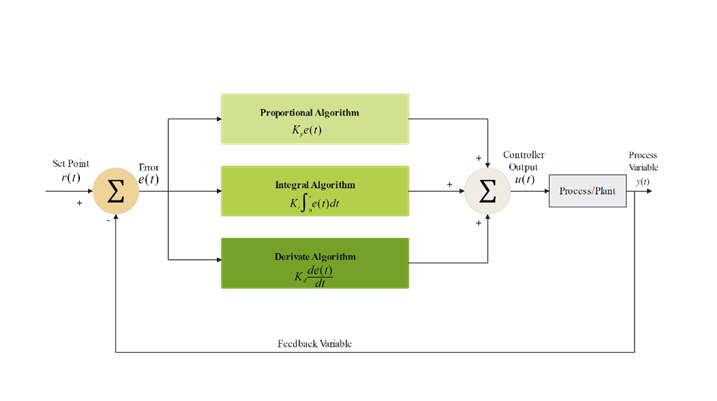
Figure 1: Block diagram of PID control algorithm

In Fig. 1, the output of the PID control algorithm is shown in equation (1).

\( u(t)={K_{p}}(e(t)+\frac{1}{{T_{t}}}\int _{0}^{t} e(t)dt+{T_{D}}\frac{de(t)}{dt})\ \ \ (1) \)

PID control is one of the most classical control techniques. It has the performance of simplicity and stability. Despite many emerging control techniques, PID controllers are still one of the most widely used controllers in the industry due to the simplicity of design and implementation, clarity of functionality and applicability. It has been shown that PID controllers exhibit good performance in many industrial automation and robotic systems, especially for linear systems and stable operating environments. In robot control applications, PID controllers are often used for position control, such as joint angle adjustment for robotic arms; In robot drive systems, PID is used to control the speed of the motor to keep it within a set range, such as systems for smooth movement of mobile robots and drones; The PID controller can also be used to control the force applied by the robot's end-effector, ensuring that the robot is able to accurately apply force during operations such as gripping, pushing and pulling; Bipedal or self-balancing robots (e.g., two-wheeled balance bikes) rely on PID control to maintain their balance, especially when dealing with complex motions and maintaining attitude stability; In mobile robot navigation, PID control helps the robot to move along a predetermined path, adjusting direction and speed to avoid deviation from the trajectory.

Although PID has a long history and a wide range of uses, research has shown that many PID feedback loop parameters are difficult to regulate[7]. Classical PID controllers are also unable to handle complex nonlinear systems as well as poor immunity and adaptability to external disturbances, which may lead to poor control, especially in systems with relatively large uncertainties or noise.

Optimisation of PID controllers is mainly based on making optimal adjustments for specific control applications. One of the most classical tuning methods is the Ziegler-Nichols Frequency Response Method [8][9]. Firstly, we need to determine the Ultimate Gains and Ultimate Period. The gain value is gradually increased in the closed-loop control state of the system until the system output begins to produce continuous oscillations. The gain \( {K_{u}} \) and the oscillation period \( {P_{u}} \) at this point are recorded. then the PID parameters are calculated using empirical formulas. Based on the recorded values of \( {K_{u}} \) and \( {P_{u}} \) , the empirical formulas in the Ziegler-Nichols method are applied to set the parameters of the PID controller as shown in Eqs. (2), (3), and (4):

\( {K_{p}}=0.5{K_{u}}\ \ \ (2) \)

\( {K_{p}}=0.45{K_{u}},{ T_{i}}=\frac{{P_{u}}}{1.2}\ \ \ （3） \)

\( {K_{p}}=0.6{K_{u}}, {T_{i}}=0.5{P_{u}},{ T_{d}}=0.125{P_{u}}\ \ \ （4） \)

Except for the classical tuning methods, common intelligent tuning methods includes auto-tuning[10], genetic algorithm approach [11]and model matching approach[12].

3. Modern control algorithms

In order to overcome the limitations of classical control theory, which is not applicable to ‘multi-input, multi-output’ systems, modern control theory was gradually developed in the 1950s and 1960s.

3.1. Adaptive control

The adaptive controller is based on the mathematical model of the system as shown in equation (5):

\( \dot{x}(t)=A(θ)x(t)+B(θ)u(t)\ \ \ （5） \)

In equation(5), \( x(t) \) is the system state, \( u(t) \) is the control input, \( A(θ) \) and \( B(θ) \) are system matrices that depend on unknown parameters.

The control input of the adaptive controller is shown in equation (6):

\( u(t)=-Kx(t)+{\hat{θ}^{T}}Y(t)\ \ \ （6） \)

In equation (6) \( K \) is the feedback gain, \( \hat{θ} \) is the estimated parameter, and \( Y(t) \) is the regression matrix.

The parameter \( θ \) is adjusted as shown in equation (7):

\( \dot{\hat{θ}}(t)=ΓY(t{)^{T}}e(t)\ \ \ (7) \)

In Equation (7) \( e(t) \) is the error signal, \( Γ \) is the conditioning matrix.

Stability analysis based on Lyapunov functions is commonly used in adaptive controllers.

\( V(x,\hat{θ})={x^{T}}Px+(θ-\hat{θ}{)^{T}}{Γ^{-1}}(θ-\hat{θ})\ \ \ (8) \)

where \( \hat{θ} \) is the estimated parameter, \( P \) is a positive definite matrix, and \( Γ \) is a matrix that regulates the rate of parameter updates[13].

Adaptive control algorithms are capable of dynamically adjusting the parameters of the controller, which is particularly suitable for dealing with parameter uncertainty and external perturbations in robotic systems Adaptive control can adjust the control parameters under unknown or varying dynamics, which enables the robotic arm to maintain stable trajectory tracking performance under varying loads, friction forces, and external perturbations. For instance, in articulated robots, adaptive control can adjust the torque output in real-time to ensure the accuracy of the end-effector. The block diagram of the model-referenced adaptive control structure, which is widely used in robot arm control, is shown in Fig. 2.

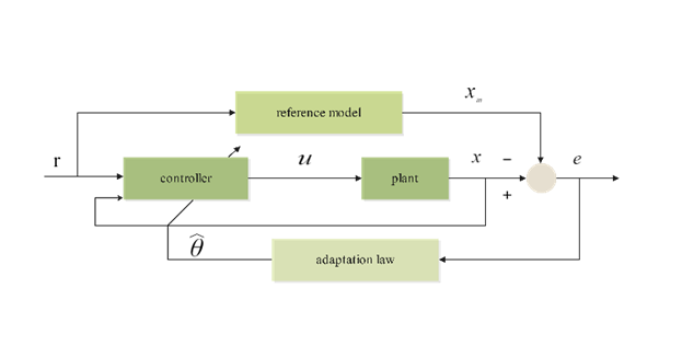
Figure 2: Block diagram of MRAC structure

By dynamically adjusting the control strategy, the adaptive control algorithm can enhance the stability of the system and ensure that the system can operate effectively under different operating conditions. In addition, the adaptive control algorithm combines the characteristics of robust control, which can maintain the stability and control performance of the system in the presence of disturbances. In UAV flight control, due to the complexity and variability of the external environment, adaptive control can effectively deal with these perturbations. In practical applications, the combination of adaptive control and sliding mode control can enhance the robustness of UAVs in uncertain environments and ensure their flight stability and path-tracking capability. Adaptive control algorithms rely on real-time adjustment of control parameters, and by improving the self-tuning algorithm (e.g., using gradient descent or Kalman filtering), the control parameters can be adjusted faster and more accurately to adapt to changes in the dynamic environment. For example, in the adaptive Kalman filter proposed in literature [14], the Kalman filter adjusts the variance of the measurement noise through a covariance matching mechanism so that the estimated residuals of the filter match the theoretical covariance. When there is uncertainty or error in the system model or measurement model, the Kalman filter can adjust the gain matrix of the filter in real-time according to the difference between the actual covariance of the innovation sequence and the theoretical covariance. This adjustment process reduces the impact of model errors on control performance and makes the system more robust.

3.2. Sliding Mode Control

The principle of sliding mode control is to design the switching hyperplane of the system according to the desired dynamic characteristics of the system, and to make the system state converge from outside the hyperplane to the switching hyperplane through the sliding mode controller. The system state model is shown in equation (9):

\( \dot{x}(t)=f(x(t),u(t))+d(t)\ \ \ (9) \)

In Equation (9), \( x(t) \) is the system state vector, \( u(t) \) is a control input, \( f(x(t),u(t)) \) is a known nonlinear function, and \( d(t) \) is an external perturbation.

Construct the sliding mould surface \( S(X) \) as a linear combination of state variables:

\( S(X)=Cx\ \ \ (10) \)

\( C \) in Equation (10) is the design matrix. For the tracking control problem, the sliding mould surface can be defined as a function of the error state:

\( S(x)=e(t)=x(t)-{x_{d}}(t)\ \ \ (11) \)

The control objective is to make \( e(t)→0 \) , that is, the system state \( x(t) \) , tracks the desired state \( {x_{d}}(t) \) .

By controlling the input \( u(t) \) , the state of the system is made to converge to and remain on the sliding mode surface. Commonly used sliding mode convergence laws are:

Constant rate convergence law:

\( \dot{S}(x)=-ksign(S(x))\ \ \ (12) \)

The law of exponential convergence:

\( \dot{S}(x)=-λS(x)-ksign(S(x))\ \ \ (13) \)

In equations (12) and (13) k and λ are positive control parameters, \( sign(S(x)) \) is a sign function.

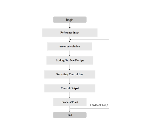
Figure 3: Flowchart of sliding mode control algorithm

Sliding mode control algorithms are capable of handling uncertainty and nonlinear systems with strong anti-interference capability. In complex situations, mobile robots may be disturbed by uneven terrain, obstacles and sensor errors. Sliding mode control is frequently used in path tracking and attitude control of mobile robots by dynamically adjusting the control law to ensure that the robot can accurately perform the intended trajectory and task. Although the pure SMC strategy has the advantage of simplicity and robustness, its main drawback is jitter, which is a high-frequency oscillation that occurs during the control process, leading to inaccurate system performance and potentially resulting in energy loss .In recent years, new mechanisms such as higher order sliding mode, terminal SMC and adaptive SMC have been introduced to mitigate the jitter problem.For example, the higher-order sliding mode control, which extends the first-order sliding mode control, controls the sliding mode surface at higher-order derivatives by introducing higher-order derivative terms, which reduces the jitter phenomenon of the system and makes the control system smoother while maintaining robustness. Although these new SMC methods provide good dynamical properties, the theoretical proof analyses of finite-time convergence and stability remain open issues due to the introduction of non-smoothness and discontinuity terms [15].

3.3. H∞ control

Since Zames proposed H∞ control synthesis, significant progress has been made in this field. The method has many theoretical advantages, such as high perturbation rejection capability and high stability, and has been widely used to solve a variety of practical and theoretical problems[9].

The H∞-based formulation of the robust control problem is shown in Fig. 4. Where 𝑤 is the vector of all perturbation signals, 𝑧 is the cost signal containing all errors, 𝑣 is the vector containing the measurement variables, and 𝑢 is the vector of all control variables.

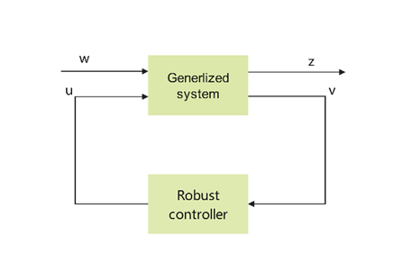
Figure 4: Robust control problem

From the literature[16], it is known that usually H∞ controllers use a combination of two transfer functions to divide the complex control problem into two independent parts, one for dealing with stability and the other for dealing with performance. The sensitivity function 𝑆 and the complementary sensitivity function 𝑇 are the parts required for controller synthesis and are defined as shown in equations. (14) and (15).

\( S=\frac{1}{1+GK}\ \ \ （14） \)

\( T=\frac{GK}{1+GK}\ \ \ （15） \)

Our goal is to find a controller 𝐾,which generates a control signal u based on the information in 𝑣 to counteract the effect of 𝑤 on 𝑧, thus minimising the number of paradigms from 𝑤 to 𝑧 in the closed-loop system such that

\( ∣∣{T_{zω}}∣{∣_{∞}}≤γ\ \ \ （16） \)

where \( {T_{zω}} \) is the transfer function from the perturbation \( ω \) to the output \( z \) and \( γ \) is the desired performance bound. By controlling the weighting functions of the sensitivity and complementary sensitivity functions (e.g., \( {W_{s}} \) and \( {W_{t}} \) ), the robustness and performance of the system at different frequencies can be ensured. The weighting functions \( {W_{s}} \) and \( {W_{t}} \) are used to qualify the sensitivity and complementary sensitivity to ensure the stability of the system over a set frequency range. A common weighting function design method is the Loop Shaping technique.

H∞ control has a strong ability to deal with uncertainty and nonlinear systems, can effectively suppress perturbations, to ensure high stability of system performance; it isapplicable to vibration suppression of flexible connecting rods, but its design and implementation process is more complex, computationally intensive [16][17][18].Due to the high degree of uncertainty and nonlinear characteristics of underwater environments, H∞ control has significant advantages in the navigation and motion control of underwater robots. By designing the H∞ controller, it can effectively respond to the perturbations of environmental factors such as water current changes and pressure fluctuations to ensure that the underwater robot can perform its tasks stably.

4. Intelligent control algorithms

As some complex systems may not be able to use accurate mathematical models to describe, the classical control theory and modern control theory will face serious challenges, the United States Purdue University Department of Electrical Engineering, Professor Fu Jingsun in the 1970s for the first time put forward the concept of ‘intelligent control’. Intelligent control, as a product of the intersection of artificial intelligence and automatic control, is a new field of automatic control science.

4.1. Neural Network Control

BP neural network is a typical nonlinear algorithm, which consists of an input layer, a hidden layer (also called intermediate layer) and an output layer , where the hidden layer has one or more layers, and the connection status of the nodes between the layers is reflected by the weights.

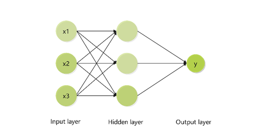
Figure 4: Schematic diagram of neural network

In Fig. 4, the output of the neural network can be represented as:

\( y=f(\sum _{i=1}^{n} {w_{i}}{x_{i}}+b)\ \ \ (17) \)

where \( y \) is the output, f is the activation function, \( {w_{i}} \) is the weight matrix, \( {x_{i}} \) is the input vector, and \( b \) is the bias term[19]. The learning process of the parameters in the neural network controller is shown below:

1. Error Calculation:

The mean square error (MSE) function was used to calculate the error in the output layer:

\( E=\frac{1}{2}\sum _{i=1}^{n}( {y_{target}}-{y_{actual}}{)^{2}}\ \ \ (18) \)

where \( E \) is the total error, \(  {y_{target}} \) is the target output, and \( {y_{actual}} \) is the actual output.

2. Backpropagation:

Backpropagate the error and update the weights layer by layer from the output layer to the hidden layer.

1) Weight update of the output layer:

\( Δw=-η\frac{∂E}{∂w}\ \ \ (19) \)

The formula \( η \) is the learning rate, which controls the magnitude of each adjustment of the weights. The partial derivative formula is:

\( \frac{∂E}{∂w}=({y_{actual}}-{y_{target}}){f^{ \prime }}(z)x\ \ \ (20) \)

where \( {f^{ \prime }}(z) \) is the derivative of the activation function and \( x \) is the input.

2) Weight update of the hidden layer:

\( {δ_{j}}=\frac{∂E}{∂{y_{j}}}\cdot {f^{ \prime }}({z_{j}})\ \ \ (21) \)

where \( {δ_{j}} \) is the error of the hidden layer neuron

3. Weight Update:

After each iteration, new weight updates are applied to the network, which ultimately results in a decreasing output error:

\( {W_{new}}={W_{old}}-η\frac{∂E}{∂W}\ \ \ (22) \)

Through repeated iterations, BP neural networks can gradually learn reasonable weight configurations in complex nonlinear relationships and achieve input-to-output mapping.

Neural network control algorithms are suitable for dealing with system designs that lack knowledge of system dynamics and can avoid complex mathematical modelling problems. It can be used for mobile robot path planning and navigation, especially when dealing with diverse obstacles and uncertainties in dynamic environments. Through learning and adaptive capabilities, neural networks can optimise robot motion control strategies and improve the accuracy and robustness of path tracking. Neural network control is used in service robots and exoskeleton systems to enhance the accuracy of human-robot interaction. For example, in exoskeleton robots, neural network control improves wearer comfort and safety by adaptively adjusting the control strategy to ensure precise matching with the user's movements.

However, the performance of small-scale neural networks in practical applications is unsatisfactory, and large-scale networks are more computationally complex and require a lot of computational time; the performance may be less than optimal in the presence of uncertainties and disturbances.

4.2. Fuzzy Control

Fuzzy control is an intelligent control method based on fuzzy set theory, fuzzy linguistic variables and fuzzy logic reasoning, which utilises the basic ideas of fuzzy mathematics and theoretical control methods applied to actual controllers.

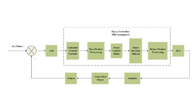
Figure 5: Block diagram of fuzzy control algorithm

As shown in Fig. 5, the fuzzy controller consists of the following four parts:

1)Fuzzification:

The input variables (exact values) are converted to the membership degree of the fuzzy set. The membership function \( {μ_{x}} \) describes the degree to which the input belongs to a fuzzy set with the formula:

\( {μ_{A}}(x)=\frac{x-a}{b-a}, for a≤x≤b\ \ \ (23) \)

Where a and b is the range of the fuzzy set and \( {μ_{a}}(x) \) is the membership degree of the input x to the fuzzy set A.

2)Rule base: A fuzzy rule base is created based on the experience of human experts.

3)Fuzzy Inference:

Reasoning based on fuzzy rules, e.g. rule: \( If {x_{1}} is {A_{1}} and {x_{2}} is {A_{2}}, then y is B. \) The inference formula is:

\( {μ_{B}}(y)=min{({μ_{{A_{1}}}}({x_{1}}),{μ_{{A_{2}}}}({x_{2}}))}\ \ \ (24) \)

Alternatively, the weighted average method is used:

\( {μ_{B}}(y)={ω_{1}}\cdot {μ_{{A_{1}}}}({x_{1}})+{ω_{2}}\cdot {μ_{{A_{2}}}}({x_{2}})\ \ \ (25) \)

Where, \( {μ_{B}}(y) \) is the output membership function, \( {μ_{{A_{1}}}}({x_{1}}) \) and \( {μ_{{A_{2}}}}({x_{2}}) \) are the membership functions of the input variables , \( {ω_{1}} \) and \( {ω_{1}} \) are the weights.

4)Defuzzification:

A common method used to convert fuzzy outputs into exact values is the Centre of Gravity (COG) method, Eq:

\( y=\frac{\int y\cdot {μ_{B}}(y)dy}{\int {μ_{B}}(y)dy}\ \ \ (26) \)

This formula calculates the centre of gravity of the fuzzy set and is used as the exact value of the system output.

Fuzzy control algorithms are capable of handling non-linear systems and do not require precise mathematical modelling; they are relatively simple to design and implement and can be used even by non-experts. Widely used in flexible robots, which often have to deal with complex working environments and uncertainty, fuzzy control handles these variables and enhances the flexibility and adaptability of robot operation. Fuzzy control is used for robot path planning and obstacle avoidance in uncertain environments. By means of fuzzy rules, the robot can autonomously judge variables such as distance and speed, make appropriate decisions, and improve the intelligence and robustness of navigation.

However, fuzzy control algorithms are more difficult to design complex systems, especially with a large number of input variables; performance may be unsatisfactory in the presence of uncertainty and external disturbances.

5. Conclusion

This paper focuses on the principles of PID control, adaptive control, sliding mode control, H∞ control, neural network control, fuzzy control and their applications in the field of robotics with the development of automation theory. As far as robustness and stability of robot control are concerned, PID control is difficult to deal with uncertainty and is less resistant and robust to interference; Adaptive control performs better in terms of robustness and stability in changing environments, while sliding mode control is more robust to system uncertainty and has good stability in theory but produces jitter in practical applications thus affecting stability; H∞ control has good robustness and high stability; Neural network control exhibits excellent robustness in MIMO systems, time-varying systems, and nonlinear systems, and the stability depends heavily on the training data; Fuzzy control may not perform well in the presence of uncertainty and external disturbances. Each robot control method has its own advantages and limitations. Therefore, hybrid control algorithms have emerged by combining the advantages of various methods and realising the complementarity of their strengths and weaknesses. In the future, the application of robots is becoming more and more widespread, and the environmental factors they face are more variable and unknown, and hybrid control algorithms will be widely used in the field of robot control. For such a new environment, how to decompose the control task of hybrid control, how to select the control algorithms that match each link, how to switch between the various algorithms, and how to evaluate the robustness and stability of the hybrid control methods are the focus of future research.

References

[1]. Shi, W.R., Qiao, T., Qiu, J.H. (2022). Design of a hybrid force/bit control system for a collaborative robot. Industrial Control Computers, 35(4), 3.
[2]. Patel, R., Zeinali, M., & Passi, K. (2021, May). Deep learning-based robot control using recurrent neural networks (LSTM; GRU) and adaptive sliding mode control. In Proceedings of the 8th International Conference of Control Systems, and Robotics (CDSR’21), Virtual (pp. 23-25).
[3]. Khalil, M., McGough, A. S., Pourmirza, Z., Pazhoohesh, M., & Walker, S. (2022). Machine Learning, Deep Learning and Statistical Analysis for forecasting building energy consumption—A systematic review. Engineering Applications of Artificial Intelligence, 115, 105287.
[4]. Alandoli, E. A., & Lee, T. S. (2020). A critical review of control techniques for flexible and rigid link manipulators. Robotica, 38(12), 2239-2265.
[5]. Yin, W.Z,, Lian, D.P., Li, K.Y., Zhao, G.W.(2023). Hybrid force/position control of robotic arm based on segmental adaptive. Journal of Beijing University of Aeronautics and Astronautics, 48.
[6]. Zhang, S.J., Wu, Y.K., Xie, B.C., & Zhao, J.L. (2023). Tracking control of wall-climbing robot based on hybrid control algorithm. Computer Integrated Manufacturing Systems, 29(11), 3560-3571.
[7]. Knospe, C. (2006). PID control. IEEE Control Systems Magazine, 26(1), 30-31.
[8]. Borase, R. P., Maghade, D. K., Sondkar, S. Y., & Pawar, S. N. (2021). A review of PID control, tuning methods and applications. International Journal of Dynamics and Control, 9, 818-827.
[9]. Ziegler, J. G., & Nichols, N. B. (1942). Optimum settings for automatic controllers. Transactions of the American society of mechanical engineers, 64(8), 759-765.
[10]. Ruano, A. E. B., Fleming, P. J., & Jones, D. I. (1992, May). Connectionist approach to PID autotuning. In IEE Proceedings D (Control Theory and Applications) (Vol. 139, No. 3, pp. 279-285). IET Digital Library.
[11]. Porter, B., & Jones, A. H. (1992). Genetic tuning of digital PID controllers. Electronics letters, 28(9), 843-844.
[12]. Aguirre, L. A. (1992). PID tuning based on model matching. Electronics Letters, 28(25), 2269-2271.
[13]. Yu, R.Z., Yuan, J.P., Li, J.Y. (2023). Adaptive control of large transport ships based on locust optimization algorithm. China Ship Research, 18, 1-9.
[14]. Brown, S. D., & Rutan, S. C. (1985). Adaptive kalman filtering. Journal of Research of the National Bureau of Standards, 90(6), 403.
[15]. Wu, L., Liu, J., Vazquez, S., & Mazumder, S. K. (2021). Sliding mode control in power converters and drives: A review. IEEE/CAA Journal of Automatica Sinica, 9(3), 392-406.
[16]. Bansal, A., & Sharma, V. (2013). Design and analysis of robust H-infinity controller. Control theory and informatics, 3(2), 7-14.
[17]. Axelsson, P., Helmersson, A., & Norrlöf, M. (2014). ℋ∞-Controller design methods applied to one joint of a flexible industrial manipulator. IFAC Proceedings Volumes, 47(3), 210-216.
[18]. Hu, J., Bohn, C., & Wu, H. R. (2000). Systematic H∞ weighting function selection and its application to the real-time control of a vertical take-off aircraft. Control Engineering Practice, 8(3), 241-252.
[19]. Ali, H., Chen, D., Harrington, M., Salazar, N., Al Ameedi, M., Khan, A. F., ... & Cho, J. H. (2023). A survey on attacks and their countermeasures in deep learning: Applications in deep neural networks, federated, transfer, and deep reinforcement learning. IEEE Access, 11, 120095-120130.
Cite this article
Wu,J. (2025). A Review of Research on Robot Automatic Control Technology. Applied and Computational Engineering,120,198-208.
Data availability
The datasets used and/or analyzed during the current study will be available from the authors upon reasonable request.
Disclaimer/Publisher's Note
The statements, opinions and data contained in all publications are solely those of the individual author(s) and contributor(s) and not of EWA Publishing and/or the editor(s). EWA Publishing and/or the editor(s) disclaim responsibility for any injury to people or property resulting from any ideas, methods, instructions or products referred to in the content.
About volume
Volume title: Proceedings of the 5th International Conference on Signal Processing and Machine Learning
© 2024 by the author(s). Licensee EWA Publishing, Oxford, UK. This article is an open access article distributed under the terms and
conditions of the Creative Commons Attribution (CC BY) license. Authors who
publish this series agree to the following terms:
1. Authors retain copyright and grant the series right of first publication with the work simultaneously licensed under a Creative Commons
Attribution License that allows others to share the work with an acknowledgment of the work's authorship and initial publication in this
series.
2. Authors are able to enter into separate, additional contractual arrangements for the non-exclusive distribution of the series's published
version of the work (e.g., post it to an institutional repository or publish it in a book), with an acknowledgment of its initial
publication in this series.
3. Authors are permitted and encouraged to post their work online (e.g., in institutional repositories or on their website) prior to and
during the submission process, as it can lead to productive exchanges, as well as earlier and greater citation of published work (See
Open access policy for details).