1. Introduction

High-order strict feedback systems [1] are a class of nonlinear systems with a wide range of applications, widely existing in industrial control and engineering systems. However, due to the system complexity and uncertainty [2], it is challenging to design efficient control algorithms. Although the traditional backstepping method [3] can effectively solve some problems, its inherent computational complexity explosion problem limits its practical application. To this end, researchers have proposed a variety of improved schemes to improve the performance and computational efficiency of the controller.

Command filtering [4] has been widely used in the control of nonlinear systems in recent years as a tool to simplify controller design. By filtering the complex virtual control signal, it avoids the calculation problem of high-order derivatives in backstepping method. However, the command filter introduces additional filtering errors [5], which may have a negative impact on the control performance of the system. Therefore, how to design an effective filtering error compensation mechanism has become an important research direction.

Radial basis function neural network [6] (RBFNN) shows significant advantages in dealing with the uncertainty of nonlinear systems because of its powerful function approximation ability. By modeling and approximating unknown nonlinear functions [7], the problems caused by modeling errors and uncertainties in control system design can be effectively solved. However, the control method of combining neural networks with command filters needs to be further studied and improved.

Based on the above research background, this paper proposes an adaptive control method that fuses command filter, filtering error compensation mechanism and radial basis function neural network. Specifically, the main contributions of this dissertation include: 1. The command filter is used to simplify the generation process of virtual control signals and solve the problem of computational complexity explosion; 2. The filtering error compensation mechanism is designed to reduce the impact of the error on the closed-loop system performance. 3. The system uncertainty is approximated and compensated based on radial basis function neural network to improve the control accuracy and robustness of the system.

The structure of this paper is as follows: The second part describes the research problem of high-order strict feedback nonlinear systems, and introduces the related basic theory. The third part introduces the design process of the controller in detail. In the fourth part, the controller performance is verified by simulation analysis. Section 5 concludes this work and looks forward to future research directions.

2. Problem description and introduction

Consider the following high-order strict feedback nonlinear system:

\( \begin{cases}\begin{matrix}{\dot{x}_{i}}={g_{i}}({\bar{x}_{i}}){x_{i+1}}+{f_{i}}({\bar{x}_{i}}), \\ {\dot{x}_{n}}={g_{n}}({\bar{x}_{n}})u+{f_{n}}({\bar{x}_{n}}), \\ y={x_{1}}, \\ \end{matrix}\end{cases} \) (1)

where \( i=1,⋯,N \) , \( {\bar{x}_{i}}=[{x_{1}},⋯,{x_{i}}] \) are system states, \( {g_{i}}({\bar{x}_{i}}) \) are system gain functions, \( {f_{i}}({\bar{x}_{i}}) \) are the unknown functions, represent the model uncertainties, \( {u_{i}} \) and \( {y_{i}} \) represent the output signals of the controller and the controlled system (1), respectively.

Lemma 1 [7]: The structure of a radial basis function neural network used as a function approximator is \( {θ^{T}}ξ(x) \) , where \( ξ(x)=[{ξ_{1}}(x),ξ(x{)_{2}},⋯,{ξ_{n}}(x)] \) is a vector with adjustable parameters. Usually \( {ξ_{i}}(x) \) are chosen as the Gaussian function \( {ξ_{i}}(x)=exp{[\frac{-{(x-{μ_{i}})^{T}}(x-{μ_{i}})}{ς_{i}^{2}}]} \) , \( i=1,⋯,n \) , and denote the center vector \( {μ_{i}} \) and kernel width \( {ς_{i}} \) of the Gaussian function. The unknown nonlinear function can be expressed as

\( f(x)={θ^{*T}}ξ(x)+{δ^{*}} \) (2)

where \( {θ^{*}} \) is the unknown optimal weight vector, \( {δ^{*}} \) is the minimum approximation error, satisfies \( |{δ^{*}}|≤δ \) , \( δ \) is an arbitrarily small positive constant. In addition, the constant \( θ \) is defined as the norm of the weight vector \( Θ \) .

Lemma 2 [8]: Introduce the command filter as

\( \begin{cases}\begin{matrix}{\dot{z}_{1}}=β{z_{2}} \\ {\dot{z}_{2}}=-2γβ{z_{2}}-β({z_{1}}-α), \\ \end{matrix}\end{cases} \) (3)

where \( {z_{1}} \) and \( {z_{2}} \) are the output signals of the command filter, \( α \) are the input signals of the command filter, \( γ \) and \( β \) represent the design parameters. By adjusting the parameters, the filtering error satisfies \( |{z_{1}}-α|≤χ \) , \( χ \) is an arbitrarily small positive constant. In order to eliminate the negative impact of the filtering error caused by the command filter on the tracking error, the following filtering error compensation mechanism is designed.

\( \begin{cases}\begin{matrix}{\dot{φ}_{1}}=a{φ_{2}}+b({z_{1,1}}-{α_{1}})-c{φ_{1}}, \\ {\dot{φ}_{i}}=a{φ_{i+1}}+b({z_{i,1}}-{α_{i}})-a{φ_{i-1}}-c{φ_{i}}, \\ {\dot{φ}_{n}}=-c{φ_{n}}-a{φ_{n-1}}, \\ \end{matrix}\end{cases} \) (4)

where \( {φ_{i}} \) are the filtering error compensation signals, \( a \) , \( b \) and \( c \) are the design parameters.

To discuss the convergence of the error compensation system, the Lyapunov function is designed to be \( {V_{c}}=\sum _{i=1}^{n}\frac{φ_{i}^{2}}{2} \) , and its derivative in the time domain is

\( {\dot{V}_{c}}=-c\sum _{i=1}^{n}φ_{i}^{2}+b\sum _{i=1}^{n-1}{φ_{i}}({z_{i,1}}-{α_{i}}) \) (5)

It follows from Young's inequality that

\( {φ_{i}}({z_{i,1}}-{α_{i}})≤\frac{φ_{i}^{2}}{2}+\frac{{χ^{2}}}{2} \) (6)

Equation (5) can be rewritten as

\( {\dot{V}_{c}}≤-\bar{c}{V_{c}}+\bar{b} \) (7)

where \( \bar{c}=2c \) , \( \bar{b} \) is a positive constant and satisfies \( \bar{b}≥b(n-1)\frac{(φ_{i}^{2}+{χ^{2}})}{2} \) . By integrating both sides of the above equation, one obtains

\( 0≤{V_{c}}(t)≤\frac{\bar{b}}{\bar{c}}+({V_{c}}(0)-\frac{\bar{b}}{\bar{c}}){e^{-\bar{c}t}} \) (8)

Obviously \( \underset{t→∞}{lim}{V_{c}}(t)=\frac{\bar{b}}{\bar{c}} \) , it means that \( \underset{t→∞}{lim}|{φ_{i}}(t)|=\sqrt[]{\frac{2\bar{b}}{\bar{c}}} \) ; Moreover, the size of the compensation signal can be adjusted by adjusting the constant \( \bar{c} \) . In summary, the compensation signal \( {φ_{i}} \) is asymptotically convergent.

3. Controller design

The reference signal \( {y_{r}} \) (step 1) and the virtual control signal \( {α_{i}} \) are passed through the command filter to obtain the output signal \( {z_{i,1}} \) . The tracking error before and after compensation is defined as \( {e_{i}}={x_{i}}-{z_{i,1}} \) and \( {S_{i}}={e_{i}}-{φ_{i}} \) , respectively, and \( {φ_{i}} \) is the filtering error compensation signal.

The Lyapunov function is designed as

\( {V_{i}}=\frac{1}{2}S_{i}^{2}+\frac{1}{2{h_{i}}}\widetilde{Θ}_{i}^{2} \) (9)

where \( {\widetilde{Θ}_{i}} \) is the estimation error.

Taking the derivative of Eq. 9 gives

\( {\dot{V}_{i}}={S_{i}}{\dot{S}_{i}}+\frac{1}{{h_{i}}}{\widetilde{Θ}_{i}}{\dot{\widetilde{Θ}}_{i}} \)

\( ={S_{i}}({g_{i}}{x_{i+1}}+{f_{i}}-{\dot{z}_{i,1}}-{\dot{φ}_{i}})-\frac{1}{{h_{i}}}{\widetilde{Θ}_{i}}{\dot{\hat{Θ}}_{i}} \) (10)

Because the system function \( {f_{i}} \) is unknown,

\( {f_{i}}({\bar{x}_{i}})=θ_{i}^{*T}{ξ_{i}}({\bar{x}_{i}})+δ_{i}^{*} \) (11)

is obtained with the help of the approximation ability of the neural network, where \( θ_{i}^{*} \) is the optimal weight vector, \( δ_{i}^{*} \) is the minimum approximation error, and \( {ξ_{i}}({x_{i}}) \) is a vector-valued function.

And then it follows from Young's inequality

\( {S_{i}}{f_{i}}={S_{i}}\hat{θ}_{i}^{T}{ξ_{i}}({\bar{x}_{i}})+{S_{i}}{δ_{i}} \)

\( ≤\frac{S_{i}^{2}{Θ_{i}}ξ_{i}^{T}{ξ_{i}}}{2ε_{i}^{2}}+\frac{ε_{i}^{2}}{2}+\frac{S_{i}^{2}}{2}+\frac{δ_{m}^{2}}{2} \) (12)

where \( {ε_{i}} \) is any positive constant and \( {δ_{m}} \) represents the upper bound of the approximation error.

Equation (10) can be rewritten as

\( {\dot{V}_{i}}={S_{i}}({g_{i}}{x_{i+1}}+{f_{i}}-{\dot{z}_{i,1}}-{\dot{φ}_{i}})-\frac{1}{{h_{i}}}{\widetilde{Θ}_{i}}{\dot{\hat{Θ}}_{i}} \)

\( ≤{g_{i}}{S_{i}}{x_{i+1}}+\frac{S_{i}^{2}{Θ_{i}}ξ_{i}^{T}{ξ_{i}}}{2ε_{i}^{2}}+\frac{S_{i}^{2}}{2}+\frac{ε_{i}^{2}}{2}+\frac{δ_{m}^{2}}{2}-{S_{i}}{\dot{z}_{i,1}}-{S_{i}}{\dot{φ}_{i}}-\frac{1}{{h_{i}}}{\widetilde{Θ}_{i}}{\dot{\hat{Θ}}_{i}} \) (13)

Next, the virtual control signal is designed to be

\( {α_{i}}=(-{k_{i}}{S_{i}}-\frac{{S_{i}}{\hat{Θ}_{i}}ξ_{i}^{T}{ξ_{i}}}{2ε_{i}^{2}}-\frac{{S_{i}}}{2}+{\dot{z}_{i,1}}+{\dot{φ}_{i}})/{g_{i}} \) (14)

Substituting (14) into (13) yields

\( {\dot{V}_{i}}≤-{k_{i}}S_{i}^{2}+\frac{S_{i}^{2}{\widetilde{Θ}_{i}}ξ_{i}^{T}{ξ_{i}}}{2ε_{i}^{2}}-\frac{1}{{h_{i}}}{\widetilde{Θ}_{i}}{\dot{\hat{Θ}}_{i}}+\frac{ε_{i}^{2}}{2}+\frac{δ_{m}^{2}}{2} \) (15)

The adaptive law is designed to be

\( {\dot{\hat{Θ}}_{i}}=\frac{{h_{i}}S_{i}^{2}ξ_{i}^{T}{ξ_{i}}}{2ε_{i}^{2}}-{σ_{i}}{\hat{Θ}_{i}} \) (16)

Substituting equation (16) into (15) yields

\( {\dot{V}_{i}}≤-{k_{i}}S_{i}^{2}+{σ_{i}}\frac{{\hat{Θ}_{i}}{\widetilde{Θ}_{i}}}{{h_{i}}}+\frac{ε_{i}^{2}}{2}+\frac{δ_{m}^{2}}{2} \) (17)

Because \( \frac{{σ_{i}}{\hat{Θ}_{i}}{\widetilde{Θ}_{i}}}{{h_{i}}}≤\frac{{σ_{i}}Θ_{i}^{2}}{2{h_{i}}}-\frac{{σ_{i}}\widetilde{Θ}_{i}^{2}}{2{h_{i}}} \) , we get

\( {\dot{V}_{i}}≤-{k_{i}}S_{i}^{2}-\frac{{σ_{i}}\widetilde{Θ}_{i}^{2}}{2{h_{i}}}+\frac{{σ_{i}}Θ_{i}^{2}}{2{h_{i}}}+\frac{ε_{i}^{2}}{2}+\frac{δ_{m}^{2}}{2} \)

\( ≤-{λ_{i}}{V_{i}}+{η_{i}} \) (18)

where \( {λ_{i}}=min{\lbrace 2{k_{i}},{σ_{i}}\rbrace } \) and \( {η_{i}}=\frac{ε_{i}^{2}}{2}+\frac{δ_{m}^{2}}{2}+\frac{{σ_{i}}Θ_{i}^{2}}{2{h_{i}}} \) are positive constants. Similarly, at Step n, the actual control signal and the corresponding adaptive law \( {\dot{\hat{Θ}}_{n}} \) are designed as

\( \begin{cases}\begin{matrix}u=(-{k_{n}}{S_{n}}-\frac{{S_{n}}{\hat{Θ}_{n}}ξ_{n}^{T}{ξ_{n}}}{2ε_{n}^{2}}-\frac{{S_{n}}}{2}+{\dot{z}_{n,1}}+{\dot{φ}_{n}})/{g_{n}} \\ {\dot{\hat{Θ}}_{n}}=\frac{{h_{n}}S_{n}^{2}ξ_{n}^{T}{ξ_{n}}}{2ε_{n}^{2}}-{σ_{n}}{\hat{Θ}_{n}} \\ \end{matrix}\end{cases} \) (19)

Integrating both sides of equation (18) yields

\( 0≤{V_{i}}(t)≤\frac{{η_{i}}}{{λ_{i}}}+({V_{i}}(0)-\frac{{η_{i}}}{{λ_{i}}}){e^{-{λ_{i}}t}} \) (20)

Obviously \( \underset{t→∞}{lim}{V_{i}}(t)=\frac{{η_{i}}}{{λ_{i}}} \) , this means as well as \( \underset{t→∞}{lim}|{\widetilde{Θ}_{i}}(t)|≤\sqrt[]{\frac{2{h_{i}}{η_{i}}}{{λ_{i}}}} \) ; Moreover, the error convergence range can be adjusted by adjusting the constant \( {λ_{i}} \) . In summary, the compensated tracking error \( {S_{i}} \) as well as the estimation error \( {\widetilde{Θ}_{i}} \) converge asymptotically.

4. Simulation analysis

The following nonlinear system is considered for simulation analysis

\( \begin{cases}\begin{matrix}{\dot{x}_{1}}={g_{1}}{x_{2}}+{f_{1}}({x_{1}}), \\ {\dot{x}_{2}}={g_{2}}u+{f_{2}}({x_{1}}+{x_{2}}), \\ y={x_{1}}, \\ \end{matrix}\end{cases} \) (21)

where \( {g_{1}}={g_{2}}=1 \) , \( {f_{1}}({x_{1}})=2x_{1}^{2} \) and \( {f_{2}}({x_{1}},{x_{2}})={x_{1}}+{cos{x}_{2}} \) .

The control signal and the adaptation law are designed as

\( \begin{cases}\begin{matrix}{α_{1}}=(-{k_{1}}{S_{1}}-\frac{{S_{1}}{\hat{Θ}_{1}}ξ_{1}^{T}{ξ_{1}}}{2ε_{1}^{2}}-\frac{{S_{1}}}{2}+{\dot{z}_{1,1}}+{\dot{φ}_{1}})/{g_{1}} \\ u=(-{k_{2}}{S_{2}}-\frac{{S_{2}}{\hat{Θ}_{2}}ξ_{2}^{T}{ξ_{2}}}{2ε_{2}^{2}}-\frac{{S_{2}}}{2}+{\dot{z}_{2,1}}+{\dot{φ}_{2}})/{g_{2}} \\ {\dot{\hat{Θ}}_{i}}=\frac{{h_{i}}S_{i}^{2}ξ_{i}^{T}{ξ_{i}}}{2ε_{i}^{2}}-{σ_{i}}{\hat{Θ}_{i}},i=1,2 \\ \end{matrix}\end{cases} \) (22)

The filtering error compensation system is described as follows:

\( \begin{cases}\begin{matrix}{\dot{φ}_{1}}=a{φ_{2}}+b({z_{1,1}}-{y_{r}})-c{φ_{1}}, \\ {\dot{φ}_{2}}=a{φ_{3}}+b({z_{2,1}}-{α_{1}})-a{φ_{1}}-c{φ_{2}}, \\ {\dot{φ}_{3}}=-c{φ_{3}}-a{φ_{2}}. \\ \end{matrix}\end{cases} \) (23)

The reference signal is \( {y_{r}}=sin{(t)} \) , the initial values of all variables are set to 0, the number of nodes of the neural network is chosen to be 30, and the kernel width is set to be 3. The command filter parameters are set to \( {γ_{i}}=2 \) , \( {β_{i}}=50 \) . The parameters of the filtering error compensation mechanism are chosen as \( a=3 \) , \( b=3 \) , \( c=5 \) . The parameters of the controller and the adaptive law are chosen as \( {k_{1}}=5 \) , \( {k_{2}}=20 \) , \( {ε_{1}}=1 \) , \( σ=0.1 \) , \( {h_{1}}={h_{2}}=20 \) . The simulation case was run on a matlab 2022a and the results are shown in Figures 1-5.

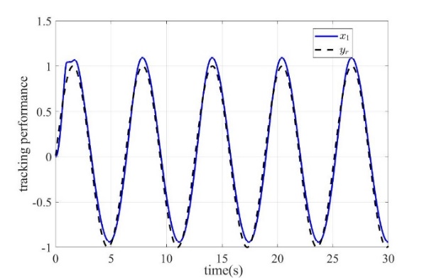
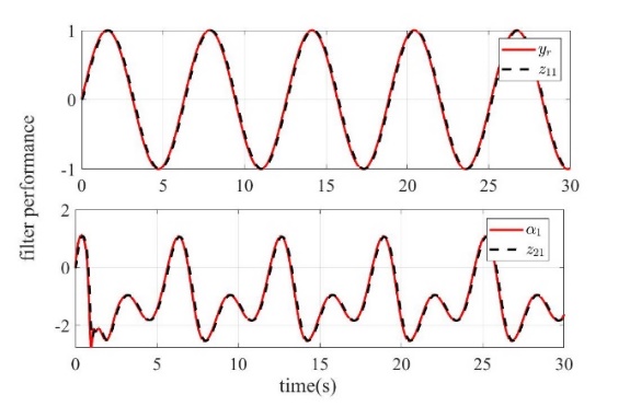
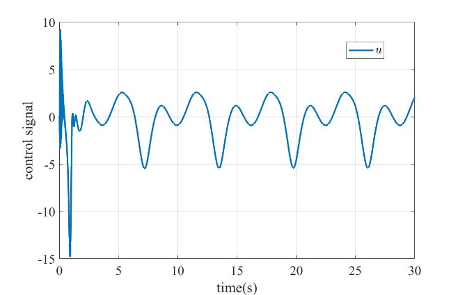
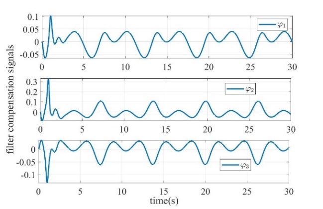
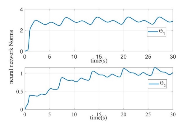
Figure 5: neural network norms

Figure 1 shows the tracking effect of the system output. It can be seen that the output of the controlled system accurately tracks the reference signal under the action of the designed neural network adaptive command filter controller. Figure 2 shows the tracking performance of the filter. It can be seen that the filter output achieves accurate tracking of the input signal. Figure 3 shows the final control signal. Fig. 4 shows the filtering error compensation signal, which completes the accurate compensation of transient error in the initial stage and tends to be stable. Fig. 5 shows the convergence of the norm of the neural network, which represents the approximation process of the neural network to the unknown function. In summary, the control strategy designed in this work achieves the desired control performance.

5. Conclusion

In this paper, the adaptive command filter control algorithm is studied for high-order nonlinear systems with strict feedback. Firstly, the command filter was used to avoid the computational complexity explosion inherent in the traditional backstepping method, and then the filtering error compensation signal was designed to alleviate the negative impact of the filtering error on the whole closed-loop system. Then radial basis function neural network is applied to deal with the system uncertainty. The final simulation results show that the proposed neural network adaptive controller can track the reference signal accurately.

References

[1]. Duan G. High-order fully actuated system approaches: Part IV. Adaptive control and high-order backstepping[J]. International Journal of Systems Science, 2021, 52(5): 972-989.
[2]. Sun J, Gu H, Zhang J, et al. Robust active finite-time control of gas compressor system surge in the presence of unmatched disturbance and uncertainty[J]. Proceedings of the Institution of Mechanical Engineers, Part I: Journal of Systems and Control Engineering, 2022, 236(5): 1049-1064.
[3]. Wang T, Zhang H, Sui S. Observer-based adaptive neural network event-triggered quantized control for active suspensions with actuator saturation[J]. Neurocomputing, 2024: 128770.
[4]. Sun G, Zhang G. Adaptive command-filtered control for system with unknown control direction caused by input backlash[J]. European Journal of Control, 2024, 76: 100962.
[5]. Zhang Y, Yao Q, Luo B, et al. Robust control of uncertain asymmetric hysteretic nonlinear systems with adaptive neural network disturbance observer[J]. Applied Soft Computing, 2024: 112387.
[6]. Wang C, Li W, Liang M. Event-triggered finite-time adaptive neural network control for quadrotor UAV with input saturation and tracking error constraints[J]. Aerospace Science and Technology, 2024, 155: 109658.
[7]. Ranjan S, Majhi S. Fixed‐Time State Observer‐Based Robust Adaptive Neural Fault‐Tolerant Control for a Quadrotor Unmanned Aerial Vehicle[J]. International Journal of Adaptive Control and Signal Processing, 2024.
[8]. Gao S, Li X, Liu J. Adaptive direct RBFNN consensus control for a class of unknown nonlinear underactuated systems[J]. International Journal of Systems Science, 2024: 1-13.
Cite this article
Li,H. (2025). Adaptive Command Filtering Control for High-order Strict Feedback Systems. Applied and Computational Engineering,129,90-96.
Data availability
The datasets used and/or analyzed during the current study will be available from the authors upon reasonable request.
Disclaimer/Publisher's Note
The statements, opinions and data contained in all publications are solely those of the individual author(s) and contributor(s) and not of EWA Publishing and/or the editor(s). EWA Publishing and/or the editor(s) disclaim responsibility for any injury to people or property resulting from any ideas, methods, instructions or products referred to in the content.
About volume
Volume title: Proceedings of the 5th International Conference on Materials Chemistry and Environmental Engineering
© 2024 by the author(s). Licensee EWA Publishing, Oxford, UK. This article is an open access article distributed under the terms and
conditions of the Creative Commons Attribution (CC BY) license. Authors who
publish this series agree to the following terms:
1. Authors retain copyright and grant the series right of first publication with the work simultaneously licensed under a Creative Commons
Attribution License that allows others to share the work with an acknowledgment of the work's authorship and initial publication in this
series.
2. Authors are able to enter into separate, additional contractual arrangements for the non-exclusive distribution of the series's published
version of the work (e.g., post it to an institutional repository or publish it in a book), with an acknowledgment of its initial
publication in this series.
3. Authors are permitted and encouraged to post their work online (e.g., in institutional repositories or on their website) prior to and
during the submission process, as it can lead to productive exchanges, as well as earlier and greater citation of published work (See
Open access policy for details).