1. Introduction

The National Basketball Association (NBA) is one of the most popular and competitive professional basketball leagues in the world. The NBA, which was established in 1946, has grown into a large, mainstream, global phenomenon that has captivated millions of fans with its intense games, extreme athleticism, and nail-biting playoff games. Iconic players such as Michael Jordan, Kobe Bryant, and Lebron James have not only impacted the NBA on the court, but also spearheaded globalization and influenced many popular trends. Akin to its iconic players, the NBA’s influence reaches further than just on the court.

Parallel to the growth and popularity of the NBA is the rise of sports betting. Betting on sports has been around for centuries, with the first documented instance of gambling being by the Ancient Greeks almost 2000 years ago during the Olympic games [1]. Now, in modern times, sports gambling has evolved into a sophisticated market with thousands of people analyzing historical data to develop models that would maximize one’s potential to win [2]. Sports gambling, in theory, has been identified as simple financial markets. Since there are only two specific defined outcomes of a match: a win or a loss. Additionally, the beginning and ending time of a matchup is very clear. Yet, regardless of the simplicity of the market, there are professionals, commonly known as bookmakers or “bookies,” who create point spreads that would drive betting actions and create a balanced betting field between two competing teams.

In sports betting, the point spread is a popular concept designed to compare two teams of varying strengths. From a betting perspective, this concept serves as a device that predicts the expected difference in the final score between two teams, acting as a tool that provides a balanced betting scenario. This, in turn, helps bettors make decisions that will attempt to maximize their winning potential. In addition, the point spread not only even the playing field from a betting perspective but also added an extra layer of complexity to the wagering process. By assigning a hypothetical final score difference between two teams, bookmakers can generate more interest on both sides of a match up. However, the assignment of a point spread should be considered in a sophisticated and well thought manner as a poor point spread may bring financial risk to the bookmaker. Contrary to the belief that point spreads should be assigned objectively, many of the current point spreads published by bookmakers may contain personal judgement that then become biases that may influence the point spreads. In addition, rather than setting a point spread to maximize the total money bet on each side of a point spread, bookmakers may also take a position regarding the outcome of the match and “exploit bettors’ biases” [3, 4].

Consequently, the objective of this research is to develop a model that can generate its own point spread based on key factors such as injuries, home court advantage, and strength of individual teams. The purpose is in hopes that by objectifying the process of generating point spreads, a more accurate and unbiased estimate of the final difference between the two teams will be presented. Thus, betters can make decisions without the biases presented in point spreads, as they are more intended for the bookmakers’ profit.

The table below reveal the primary data set used in this study, produced by using R [5]. The data set had been cleaned and merged with two primary data sets. It is also worth mentioning that the primary datasets had already properly cleaned or merged, and the process would be further illustrated in Appendix. The primary data set used for the model are the results of the 2012-2013 NBA season, which includes the date of the match, the team names and the match’s corresponding point spread, scores, score difference, location of the match, injured players, and the total number of injured players for both teams.

Table 1. Part 1 of the First 6 Rows of the Data Set:

Table 2. Part 2 of the First 6 Rows of the Data Set

Table 3. Part 3 of the First 6 Rows of the Data Set

Table 4. Part 4 of The First 6 Rows of the Data Set

Table 5. Part 5 of The First 6 Rows of the Data Set

2. Methodology

2.1. Regression Model

The three primary random factors affecting NBA competition results are: Home court advantage, injuries, and consecutive games, with the regression model is showing the relationship between score difference and these variables.

\( Predicted Score Difference = {T_{2}}- {T_{1}}+ {I_{home}}- intercept+{I_{injury}}+ {I_{consecutive}} \)

Where \( {T_{1,2}} \) is the strength of Team 1 and 2; \( I \) is the impact of three factors, respectively; \( intercept \) is the compensation of error.

2.2. Verification of Accuracy of Regression Model

To verify the accuracy of the predicted results, the r-squared value and mean absolute error (MAE) will be calculated every time a random factor that could impact NBA score result is implemented in the model. This way, it ensures that there is significance with each implementation. Finally, with the final regression model, the last 50 games of the 2012-2013 will be predicted and its MAE and r-squared would be compared with the actual point spread. This way, these measurements will indicate how more accurate the prediction of the model is than the point spread.

As mentioned, in this study there will be two measurements used to indicate the accuracy of the model: MAE and \( {r^{2}} \) . Firstly, MAE represents the average magnitude of errors in a set of predictions. As a result, MAE provides a clear metric for understanding the model's prediction accuracy. In the context of NBA score difference prediction, a lower MAE indicates that the predicted score differences closely align with the actual outcomes, signifying a more accurate model.

\( MAE=\frac{1}{n}\sum | {y_{i}}-{\hat{y}_{i}} | \)

Where \( n \) represent the total number of observations or data points, \( {y_{i}} \) represents the actual observed value for the \( i \) -th data point, and \( | {y_{i}}-{\hat{y}_{i}} | \) is the absolute error.

The other metric is the \( {r^{2}} \) . It is a statistical measure that represents the proportion of the variance in the dependent variable (score difference) that is predictable from the independent variables (team strength, home court advantage, and injuries). An r-squared value closer to 1 indicates that a higher proportion of the variance is explained by the model, suggesting a better fit [6, 7, 8].

3. Construction and Development of Regression Model for the NBA

3.1. Baseline Model: Strength of Individual Teams (T₁ & T₂)

Primarily, the model's foundation will be set as the strength of individual teams. To quantify the strength of individuals teams, the average points scored by a team (getscore) and the average points allowed (givescore) were calculated using the 2012-2013 NBA data. Specifically, “getscore” represents the mean points scored by each team across all games, while the “givescore” represents the mean points allowed by each team in those games. Then an “advantage,” variable was calculated as the difference between the two previous values. Differ from the random factors, the strength of each team is a more stable factor that represents the inherent power of a team based on its historical performances. As a result, it is used as a baseline when predicting score differences, with the random factors being adjustments to this baseline. This method also ensures that stronger teams, which would usually score more and allow fewer points on average, are accurately reflected in the model’s predictions in having a greater advantage.

\( getscore({T_{i}})= \frac{1}{{n_{i}}}\sum _{j=1}^{{n_{i}}}{score1_{ij}} \)

\( givescore({T_{i}})= \frac{1}{{n_{i}}}\sum _{j=1}^{{n_{i}}}{score2_{ij}} \)

\( advantage({T_{i}})= getscore({T_{i}})-givescore({T_{i}}) \)

\( {T_{i}} \) represents a specific team \( i \) , \( {n_{i}} \) is the total number of games played by team \( i \) , \( {score1_{ij}} \) represents the points scored by team \( i \) in game \( j \) , \( {score2_{ij}} \) represents the points allowed by team \( i \) in game \( j \) which corresponds to the score of the opponent team.

With the initial regression model, the last 50 games of the season were predicted based on the calculated team strengths. For each game, the predicted score difference was computed by taking the difference in the advantage scores between the two teams involved. These predictions were then compared to the actual score differences to evaluate the model's performance as shown in Figure 1.

Figure 1. Regression 1

In Figure 1, the comparison between the first estimation and actual score difference was visualized of the first estimation was visualized with a regression line fitted to the data. The initial model yielded an \( {r^{2}} \) value of 0.2108, which indicates that approximately 21% of the variance in the score differences was explained by the model. Additionally, the Mean Absolute Error (MAE) was calculated to be 9.5237, providing a baseline measure of the model's accuracy when implementing other random factors.

3.2. Random Factor: Home Court Advantage (I_home)

After a baseline was set for the model, the first random factor considered is home court advantage. Home court advantage reflects the varying performance of teams when playing on their home court versus when they are visitors with teams usually perform better at home than away [9]. For this model, to accurately incorporate this factor into the regression model, the strength of each team was calculated separately for home and away games.

Initially, the focus was on the games where each team were played at home. For these home games, the average points scored, and the average points allowed were computed for each team. The difference between these values provided the home court advantage, indicating how much better a team performs when playing at home compared to away. Similarly, the team's performance as visitors was also evaluated to understand their performance when playing away from home.

The results revealed that the mean score difference for home games was approximately -3.28, indicating that, on average, teams scored fewer points than they allowed when playing at home. However, this seemingly counterintuitive result reflects the calculation method, where the score difference is negative because the analysis is considering the difference from the perspective of the away team. Essentially, this means that, on average, Team 1 (the home team) scores higher when playing at home, compared to Team 2 (the away team). In fact, the mean score difference of the home games is approximately 1.67% higher than at away games, which further exacerbate the importance of implementing Home Court Advantage in the model.

The differences between home and away performances were then visualized in a Figure 2, which illustrated the score differences for each team across different conditions—home, away, and average performance. The graphical representation clearly showed the significant impact of home court advantage on team performance, with most teams exhibiting better scores at home than away.

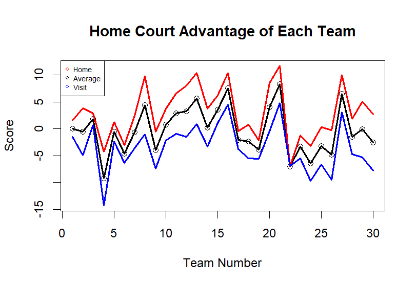
Figure 2. Home Court Advantage of Each Team

In the second stage of the model's development, the focus was initially placed on refining the predictions for games where teams played at home, before extending the analysis to include all games—both home and away. This two-part approach aimed to enhance the predictive accuracy by separately accounting for the specific advantages and disadvantages teams experience when playing on their home court versus away.

Home-Only Regression:

The first step involved analyzing only the home games to better understand the impact of home court advantage. The regression model predicted the score differences by considering the adjusted home and visit advantages for each team. The results, visualized in Figure 3, indicated a bias in the predictions. In which, the regression line demonstrated a tendency to underestimate the actual score differences, as reflected by an intercept of -5.7651. This downward bias arose because the calculation typically involved subtracting a smaller visitor advantage from a larger home advantage.

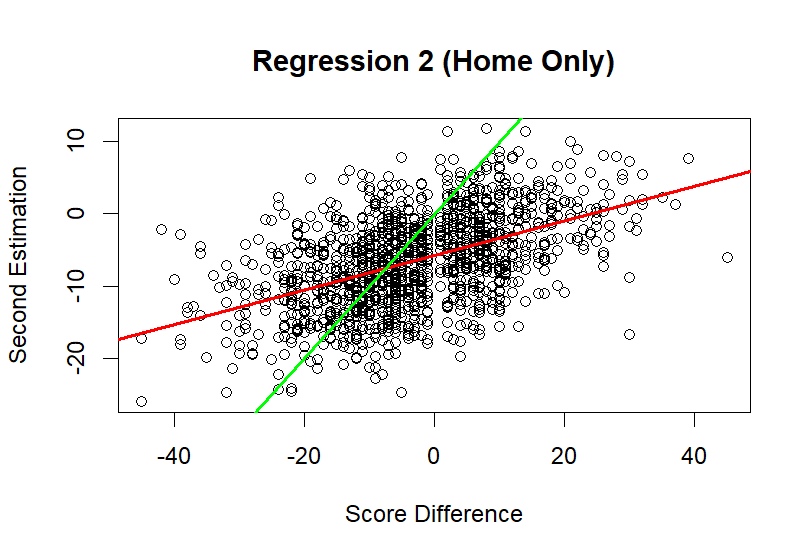
Figure 3. Regression 2 (Home Only)

To address this, a compensation adjustment was calculated, resulting in a value of approximately -3.2763. This adjustment aimed to correct the bias in future predictions, bringing them closer to the actual outcomes. The inclusion of this compensation improved the model's alignment with the real-world dynamics of NBA games, where home court advantage significantly influences the final score difference.

Overall Regression:

Extending on the insights gained from the home-only analysis, the model was then extended to include all games. This comprehensive regression model incorporated the calculated home and visit advantages for each team, along with the previously determined compensation adjustment.

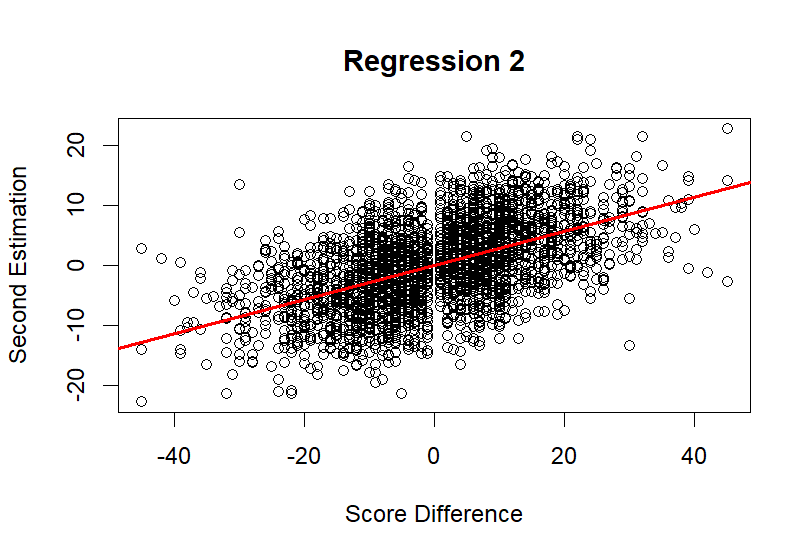
Figure 4. Regression 2

The results of this overall regression are shown in the "Regression 2" scatter plot, which displays the relationship between the predicted and actual score differences for all games. The model demonstrated a positive correlation between predictions and outcomes, with a \( {r^{2}} \) value of 0.2892, indicating that approximately 29% of the variance in score differences was explained by the model. Additionally, the Mean Absolute Error (MAE) was reduced to 8.9410, reflecting an improvement in prediction accuracy compared to earlier models.

In this extended model, the prediction process varied based on whether the game was played at home or away. For home games, the predicted score difference was calculated by subtracting the visitor's advantage from the home team's advantage, with an additional compensation adjustment. Conversely, for away games, the compensation was added to adjust the predictions accordingly.

3.3. Random Factor: Player Injury (I_Injury)

Building off the insights from previous regression models, the third regression model integrated the impact of injuries with home and visit advantages to provide a comprehensive estimation of score differences. This model considered both the number of injured players on each team and their respective home or visit advantages, alongside the previously calculated compensation adjustment.

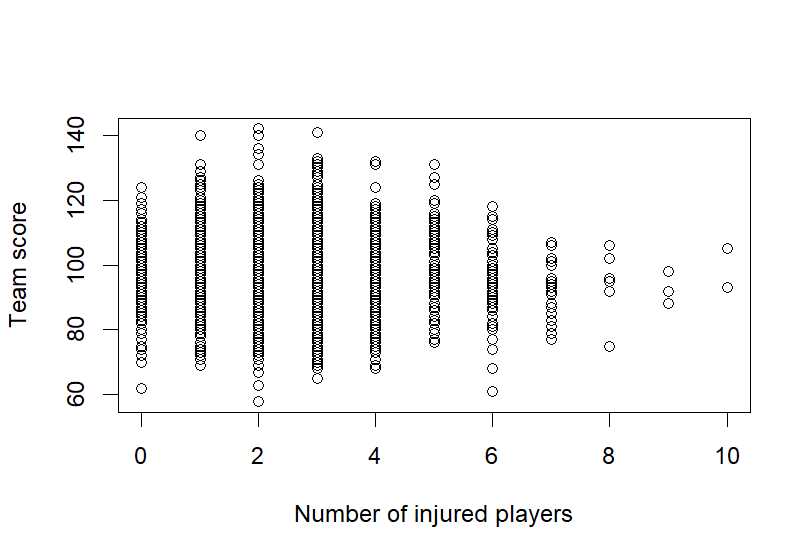
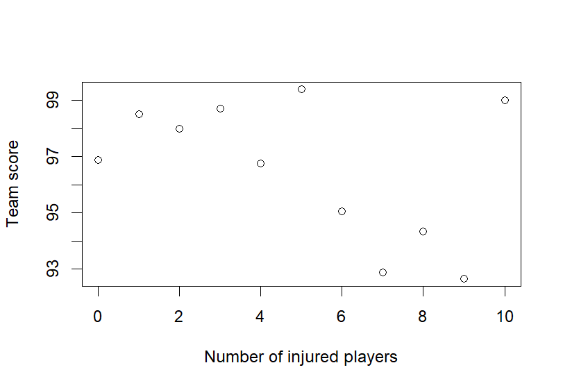
Figure 5. Impact of Injury on Scores Figure 6. Impact of Injury on Scores – Average

In Figure 5a, the graph shows the distribution of team scores across different numbers of injured players. Each dot on the scatter plot represents a game, with the x-axis indicating the number of injured players and the y-axis representing the team's score in that game. As the number of injured players increases, the plot reveals a general trend of declining team scores. Notably, the spread of scores becomes narrower as the injury count rises, indicating that teams with more injuries are more likely to score lower, and their performance becomes more predictable in a negative sense. The wide range of scores when few or no players are injured reflects the variability in team performance when nearly the full roster is available. However, as injuries accumulate, this variability decreases, often leading to consistently lower performance.

In comparison, Figure 5b takes the analysis a step further by displaying the average team score for each level of injury count. The x-axis still represents the number of injured players, but the y-axis now shows the average score that teams with that number of injuries typically achieve. The downward-sloping trend line in this plot clearly illustrates that the average score decreases as the number of injured players increases. This visual confirms that injuries have a negative, cumulative impact on team performance. This relationship suggests that even a small number of injuries can significantly reduce a team's scoring ability, and the impact becomes more pronounced as more players are sidelined. The quadratic nature of the trend line indicates that the effect of each additional injury is not linear; instead, it increases at a growing rate as the number of injuries rises.

However, during the analysis, an outlier was detected when the number of injured players reached 10, which significantly skewed the regression results. To ensure the accuracy of the model, this abnormal value was removed from the dataset. This injury impact model was then integrated into the overall regression framework to adjust the predicted score differences based on the number of injured players. For home games, the predicted score difference was calculated by adding the injury impact to the home team's advantage and subtracting the visitor's adjusted advantage. The previously calculated compensation adjustment was then applied. For away games, the process was reversed, adjusting the visitor's advantage by the impact of injuries and compensating accordingly.

To quantify this relationship, a regression equation was established:

\( Score=97.3691+0.8102 × inj-0.1778 × {inj^{2}} \)

In this equation, \( inj \) represents the number of injured players on the team. The linear term indicates that for each additional injured player, the team’s score initially decreases by approximately 0.81 points. Additionally, the quadratic term reflects the non-linear nature of the impact, showing that the negative effect of injuries on team performance intensifies as the number of injured players increases [7].

This model was then integrated into the overall regression framework to adjust the predicted score differences based on the number of injured players. For home games, the predicted score difference was calculated by adding the injury impact to the home team's advantage and subtracting the visitor's adjusted advantage. The previously calculated compensation adjustment was then applied. For away games, the process was reversed, adjusting the visitor's advantage by the impact of injuries and compensating accordingly.

Figure 7. Regression 3

With injuries’ impact on the game considered, Figure 6 shows the relationship between the final predicted score differences and the actual score differences for all games in the dataset. The scatter plot illustrates how well the model's predictions align with the actual outcomes. The red regression line, shows a positive correlation, indicating that the model's predictions are generally in line with actual results. More precisely, the model's performance was evaluated using the \( {r^{2}} \) value and Mean Absolute Error (MAE). The \( {r^{2}} \) value for this final model was calculated to be 0.2903, indicating that approximately 29% of the variance in score differences are explained by this comprehensive model. Additionally, the Mean Absolute Error (MAE) was found to be 8.9088, reflecting the model's precision in predicting game outcomes.

3.4. Random Factor: Consecutive Games (I_consecutive )

The final random factor implemented in the regression model, is the impact of consecutive games on team performance. In context, teams playing consecutive games could lead the players with fatigue, which in turn can affect a team's scoring ability. The influence of this factor is particularly significant in the NBA, where teams often play multiple games within a short period, leading to varying levels of rest between competitions.

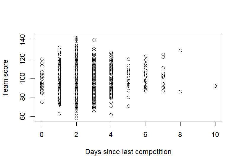
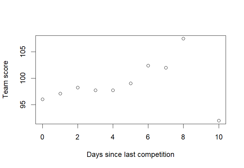
Figure 8. Impact of Consecutive Games Figure 9. Impact of Consecutive Games– Average

In Figure 7a, the graph shows the distribution of team scores based on the number of days since their last game, represented as \( datediff \) . The scatter plot indicates that as the number of rest days increases, team scores generally improve. When rest is minimal, the spread of scores is wider, suggesting that teams perform inconsistently due to fatigue. As rest days accumulate, teams tend to score higher and more consistently. An outlier at \( datediff \) = 10 was identified, where the score was lower than expected, possibly due to disruptions from an extended break. This outlier was removed from the analysis to ensure the model accurately reflects typical performance trends.

Then in Figure 7b, the graph examines this relationship by showing the average team score for each level of \( datediff \) . The trend line indicates that average scores increase with more rest, reflecting a positive relationship between rest days and performance. The effect is exponential, with each additional rest day leading to greater improvements in scores, particularly as rest days increase beyond three to five days. This highlights the cumulative benefits of rest and emphasizes the importance of considering rest periods in predicting game outcomes.

The relationship between rest days and team performance was quantified using the following regression model, created because of fitting a non-linear regression model to the data:

\( Score=0.2016 × {1.6027^{datediff}}+97.3289 \)

In this equation, \( datediff \) represents the number of days since the team's last game. The model was fitted using non-linear least squares (NLS) to account for the exponential relationship observed between rest days and scores [7]. This model indicates that as the number of days increases, the team’s score rises exponentially, reflecting the enhanced performance associated with more rest. The exponential term captures how performance improves at an increasing rate with more rest days, while the baseline score of 97.3289 represents the team’s average score with minimal rest.

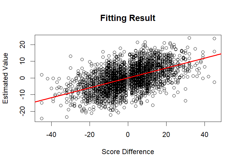
Figure 10. Fitting Result

At last, with the impact of all considered factors incorporated into the model, the final predictions were made, and the performance metrics provide a clear indication of the model’s enhanced predictive capability. The \( {r^{2}} \) value of 0.2873, which indicates that approximately 28.73% of the variance in actual score differences are explained by the model, and the Mean Absolute Error (MAE) of 8.9201, reflecting the average deviation of the model’s predictions from the actual score differences.

4. Test Results and Discussion

Finally, with all three random factors considered in the model, the accuracy of the model is tested to ensure its superior predictability when compared to the point spread. The point spread, yielded an \( {r^{2}} \) value of 0.2475 and an MAE of 9.1507. In contrast, the final regression model developed achieved an \( {r^{2}} \) value of 0.2873 and an MAE of 8.9201. With both a higher \( {r^{2}} \) value and a lower MAE, this effectively indicates that there is an improvement in predictive power over the point spread. In addition, each time a random factor was implemented in the model, there is a positive correlation with the model’s ability to generate accurate score differences. Essentially, this portrays that the factors that were implemented in the model were in fact relevant and would impact the results of the game.

Specifically, succeeding the creation of the base model, the inclusion of home court advantage increased the base model’s \( {r^{2}} \) value by approximately 0.78, which adjusted the predicted outcomes favorably for home teams that would outperform their opponents on their own court. In addition, the consideration of injury data further improved the \( {r^{2}} \) to 0.2903, as it accounted for the significant impact of player absences on team performance. Finally, incorporating rest periods between consecutive games contributed to refining the predictions for fatigued teams that often underperforms when playing back-to-back games, with the final model achieving a \( {r^{2}} \) of 0.2873. Additionally, the MAE decreased from 9.5237 in the initial model to a final MAE of 8.9201 in the final model.

In summary, the comparison of the model's performance with the point spread clearly shows that the model offers superior predictive accuracy. The improvement in both \( {r^{2}} \) and MAE underscores the value of integrating multiple relevant factors into the analysis, leading to a more detailed and accurate prediction of game outcomes. These findings suggest that the model has strong potential for practical applications when precise outcome predictions is needed.

5. Limitations

Although the regression model was shown to be more predictive than the point spread when predicting game outcomes for the 2012-2013 season. Yet, there are simplified assumptions made that may would negatively impact the accuracy of the model. For example, when considering the impact of injuries, the level of injuries was assumed the same across all players. This also implied that the model only considered when and when not a player is available to play. Yet, the potential of the negative impact an injury may bring to the player on court was not considered, nor the severity. As a result, this would potentially contribute to certain inaccuracies of the model. Additionally, another limitation of the model is its over-reliance on historical data without accounting for changes during the season. For example, sometimes NBA players are traded in the middle of the season which may have impact on the overall team strength.

6. Future Work

One potential area for future exploration can be enhancing the current regression model by adapting data from multiple NBA seasons. This way, a model with a greater data base would be more stable and consistent. In addition, this would involve gathering and cleaning data from other NBA seasons. Presumably, also assigning different weighting to different NBA set data as older NBA season results would have less of an impact on the predicament of point spread for more recent years. Moreover, one could examine how changes in team rosters, coaching strategies, or league-wide rule changes affect the model’s predictions. Understanding these dynamics could provide deeper insights into the factors that most significantly impact game outcomes. Which would ultimately contribute to a more refined model.

7. Conclusion

In conclusion, this paper has presented a regression model that demonstrated an increase of accuracy when predicting NBA score differences than the point spread. By using, MAE and \( {r^{2}} \) , the model’s precision and fit was quantified, which showed the how various random factors affected the model’s predictive capabilities. Finally, the results effectively suggested that team strength, as well as random factors such as home court advantages, injuries and consecutive games remain critical when attempting to predict a game’s outcome.

References

[1]. Matheson, V. (2021) 'An overview of the economics of sports gambling and an introduction to the symposium, ' Eastern Economic Journal, 47(1), pp. 1–8. https://doi.org/10.1057/s41302-020-00182-4.
[2]. Levitt, Steven. (2004). Why are Gambling Markets Organized so Differently from Financial Markets?. Economic Journal. 114. 223-246. 10.1111/j.1468-0297.2004.00207.x.
[3]. Feddersen, A., Humphreys, B. R. and Soebbing, B. P. (2013) 'Sentiment bias in National Basketball Association Betting, ' West Virginia University [Preprint]. http://busecon.wvu.edu/phd_economics/pdf/13-03.pdf.
[4]. Weinbach, Andrew & Paul, Rodney. (2008). Price Setting in the NBA Gambling Market: Tests of the Levitt Model of Sportsbook Behavior. International Journal of Sport Finance. 3. 137-145.
[5]. R Core Team (2024). _R: A Language and Environment for Statistical Computing_. R Foundation for Statistical Computing, Vienna, Austria. <https://www.R-project.org/>.
[6]. Fernando, J. (2024) R-Squared: Definition, Formula, Uses, and Limitations. https://www.investopedia.com/terms/r/r-squared.asp.
[7]. O’Brien, T.E. and Silcox, J.W. (2024) 'Nonlinear Regression Modelling: A Primer with Applications and Caveats, ' Bulletin of Mathematical Biology, 86(4). https://doi.org/10.1007/s11538-024-01274-4.
[8]. Schneider, A., Hommel, G. and Blettner, M. (2010) 'Linear Regression analysis, ' Deutsches Ärzteblatt International [Preprint]. https://doi.org/10.3238/arztebl.2010.0776.
[9]. Courneya, K. S., and Carron, A. V. (1992). The Home Advantage In Sport Competitions: A Literature Review. Journal of Sport and Exercise Psychology 14, 1, 13-27, available from: <https://doi.org/10.1123/jsep.14.1.13> [Accessed 23 August 2024]
[10]. NBA Injuries from 2010-2020 (2020). https://www.kaggle.com/datasets/ghopkins/nba-injuries-2010-2018.
Cite this article
Wang,Y.;Ji,H.;Dai,D. (2025). From sidelines to scoreboards: Regression modelling for predicting NBA game outcomes. Applied and Computational Engineering,131,60-71.
Data availability
The datasets used and/or analyzed during the current study will be available from the authors upon reasonable request.
Disclaimer/Publisher's Note
The statements, opinions and data contained in all publications are solely those of the individual author(s) and contributor(s) and not of EWA Publishing and/or the editor(s). EWA Publishing and/or the editor(s) disclaim responsibility for any injury to people or property resulting from any ideas, methods, instructions or products referred to in the content.
About volume
Volume title: Proceedings of the 2nd International Conference on Machine Learning and Automation
© 2024 by the author(s). Licensee EWA Publishing, Oxford, UK. This article is an open access article distributed under the terms and
conditions of the Creative Commons Attribution (CC BY) license. Authors who
publish this series agree to the following terms:
1. Authors retain copyright and grant the series right of first publication with the work simultaneously licensed under a Creative Commons
Attribution License that allows others to share the work with an acknowledgment of the work's authorship and initial publication in this
series.
2. Authors are able to enter into separate, additional contractual arrangements for the non-exclusive distribution of the series's published
version of the work (e.g., post it to an institutional repository or publish it in a book), with an acknowledgment of its initial
publication in this series.
3. Authors are permitted and encouraged to post their work online (e.g., in institutional repositories or on their website) prior to and
during the submission process, as it can lead to productive exchanges, as well as earlier and greater citation of published work (See
Open access policy for details).