1. Introduction

Landslide is a very serious natural disaster. Various phenomena can affect the stability of slopes and trigger landslides, such as high winds, rainfall, snowmelt, temperature changes, seismic shaking, volcanic activity and human activities [8]. It poses a very serious threat to human lives and also affects people’s daily lives.

Landslides include all forms of slope mass movement and may involve soil, rock, debris, organic matter, artificial fill or mixtures of these materials. These downward or outward movements can be classified into different categories based on factors such as rate of movement (ranging from a few millimeters per year to tens of meters per second), water content, and other characteristics [1]. Landslides may involve flow, sliding, tipping, falling or spreading. When landslides occur, they exhibit different combinations of these types of movement either simultaneously or during their development [8].

In order to prevent landslides in a timely manner, it is important for humans to assess the risk of landslides. When evaluating the likelihood of landslides occurring within a certain timeframe and area, it is crucial to identify the conditions that led to slope instability and the processes that initiated the movement [6]. This encompasses a large number of fac- tors, such as water content in the soil, vegetation cover, slope gradient, slope orientation, lithologic characteristics of the mountain, and elevation. Therefore, artificial Intelligence can be very effective in solving this problem.

Artificial Intelligence has applications in various aspects. It can mimic human thinking through computers or machines in order to solve some practical problems or make decisions. Artificial Intelligence is much faster than humans in this regard and gives more accurate results. Machine learning, as a branch of artificial intelligence, is more oriented to- wards autonomous learning. Machine learning can acquire knowledge from given data to achieve a predicted outcome for a particular event.

There are many types of machine learning algorithms, such as artificial neural networks, decision trees, support vector machines, and random forests [11]. The main emphasis in this article is on the application of random forests in machine learning. Random forests refer to the process of significantly improving classification accuracy by growing a set of trees and letting them vote for the most popular category. While nurturing this set of trees, the growth of each tree is controlled by generating random vectors. After having a large number of trees, they vote for the most popular cate- gory [3].

The goal of this research is to predict whether or not a landslide will occur at a given location through the application of random forests in machine learning. The prediction is based on the orientation, curvature, elevation, lithologic characteristics, vegetation index, and water content in the soil to determine if a landslide will occur. The risk level of the landslide is then assessed based on the difference in water content of the soil within one meter of the site. Each risk level corresponds to a different interval of water content. In ma- chine learning, different risk levels are represented by different colors. In the experimental process, we train the random forest with the existing dataset and continuously improve the prediction accuracy. At the same time, we calculate the attenuation of the signal paths through known models and formulas to obtain the differences in soil water content. Finally, we use Hidden Markov Chains to predict future changes in soil water content for constant risk assessment.

2. Channel model for soil with different \( mv \) communication

We assume that the signal base station is located on the surface, with the sensor placed two meters underground. The signal propagates through underground-to- aboveground(ug2ag), experiencing some attenuation. By analyzing how the signal attenuates differently in soil with varying moisture content, we can calculate the signal attenuation strength and predict the distribution of soil moisture in that area.

The Friis Equation is given as

\( Pr = PtGtGr{(\frac{λ}{4πD})^{η}} \) (1)

where η is the path loss exponent, Pr and Pt are the receiver power and transmit power, respectively, Gt is the antenna gains at the sender and Gris the antenna gains at the receiver, D is the distance between base station and sensor. However, in order to be more in line with our reality, the formula is corrected as follows[7]:

\( Pr = Pt+ Gt+ Gr - (Lug(dug) + Lag(dag) + L(R,→)) \) (2)

in which Lug(dug and Lag(dag are the loss at the underground and the aboveground portions, respectively, while L(R,→) is the refraction loss based on the propagation direction, → , i.e.,ug2ag,and we assume that L(R,→) = 0.

The underground and aboveground losses in (2) are given as:

\( Lug(dug) = 6.4 + 20logdug + 20logβ + 8.69αdug \) (3)

\( Lag(dag) = -147.6 + 10ηlogdag + 20logf \) (4)

respectively, where f is the operation frequency, α is the attenuation constant, and β is the phase shifting constant. The above- ground losses depend on the attenuation coefficient, η, which is higher than 2 due to the impacts of ground reflection. And the under- ground losses depend on the last two terms in (3),where α and β are given as:

\( α=\frac{2πc}{{λ_{0}}}\sqrt[]{\frac{{μ_{r}}{μ_{0}}{ϵ_{0}}{ϵ^{ \prime }}}{2}[\sqrt[]{1+{(\frac{{ϵ^{ \prime \prime }}}{{ϵ^{ \prime }}})^{2}}}-1]} \) (5)

\( β=\frac{2πc}{{λ_{0}}}\sqrt[]{\frac{{μ_{r}}{μ_{0}}{ϵ_{0}}{ϵ^{ \prime }}}{2}[\sqrt[]{1+{(\frac{{ϵ^{ \prime \prime }}}{{ϵ^{ \prime }}})^{2}}}+1]} \) (6)

in which ϵ′ and ϵ′′ are the real and imaginary parts of the effective soil permittivity.

In order to get a direct equation for the relationship between mv and signal transmission loss, we note that the dielectric constant of the soil is related to its mv. The dielectric constant has an approximately linear relation- ship with mv, which is given as [10]:

\( ϵ \prime = 64.14mv + 1.738 \) (7)

\( ϵ \prime \prime = 7.6mv + 1.414 \) (8)

The real and imaginary parts of the dielectric constant at different are obtained, and substituting them into (5) (6) gives the path loss of the signal at that mv.

By fitting the data, shown in Fig.1, we obtained a quadratic relationship between Pr and the of the soil as shown in Fig1.The and SSE are 0.9997 and 0.0339, respectively. The relationship is given as:

\( Pr = -4.13mv2 + 31.92mv + 61.26 \) (9)

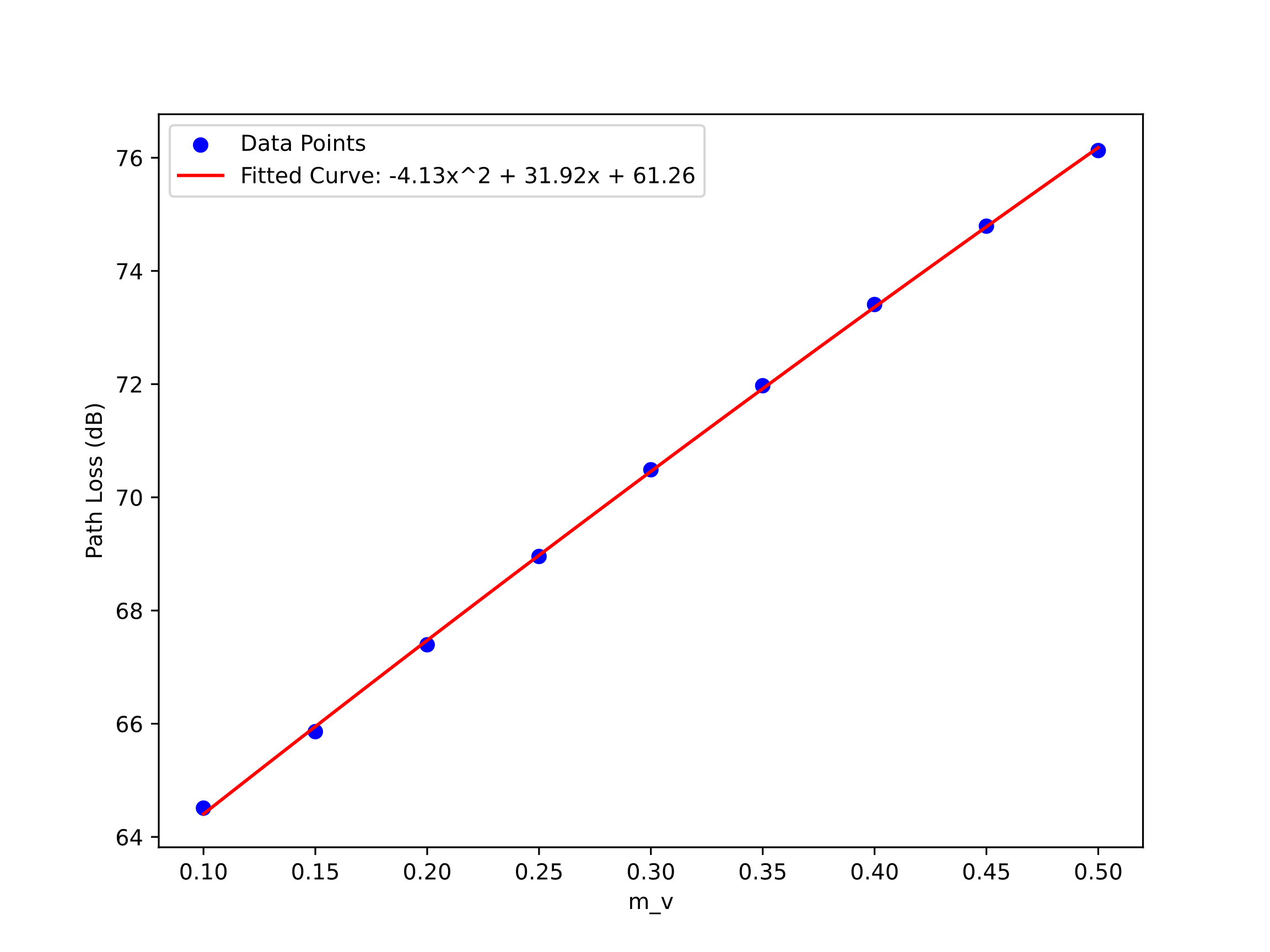
Figure 1. The relationship between path loss and mv

3. Assess risk and accuracy by using the Random Forest algorithm

When large amounts of data need to be processed, machine learning is one of the most efficient and mainstream methods. The ma- chine is divided into many large modules, Including Supervised Learning, unsupervised learning, semi-supervised learning, reinforcement learning, transduction, and learning to learn [9]. In the classification problem, supervised learning algorithms are used to learn the training dataset and produce a model, and then the logic of this part is applied to the un- labeled data [4] (that is, the testing dataset). After comparing the application of machine learning algorithms in the field of risk assessment, especially in the field of landslide, it is found that the Random Forest algorithm [5] is one of the most widely used and effective algorithms.

3.1. Data Processing

In order to ensure that the evaluation methods used in the experiment are consistent, the data sets used in this study are divided. In other words, a quantitative number of data were randomly selected from this dataset of Landslide Prediction for Muzaffarabad-Pakistan on Kaggle as training dataset and testing dataset. After testing the complete rental data, it was found that the data was not missing, so the data set was randomly divided. However, it also ensures that the training dataset contains 700 sets of data the testing dataset contains 100 sets of data, and each set of data contains 12 influencing factors to be studied.

3.2. Decision trees

The running logic of the random forest algorithm is to input a set of training datasets and build decision trees according to the content to be evaluated. For the dataset used in this paper, Landslide in Muzaffarabad- Pakistan, he looked at whether a landslide was an influential factor at the center of an area. Therefore, for this database, each small decision tree is divided according to these 12 influencing factors.

3.3. Parameter setting and accuracy

The accuracy of the Random Forest algorithm depends on the joint action of the Decision Tree Classifier and the Random Forest Classifier. When setting the parameters of the decision tree, there was no problem with weight setting because the experiment measured 12 influencing factors fairly. Therefore, for the random forest classifier of this experiment, the parameter that needs to be adjusted most is the maximum depth. Depth determines the complexity of the algorithm [2]. If the maximum depth is too small, the model will not fit well, but if the maximum depth is too large, the model will over fit. An- other factor that greatly affects the decision tree classifier is the minimum sample split, which sets the minimum number of samples required within each split node. In addition, some parameters also have a crucial impact on the accuracy of the Random Forest algorithm. n estimator This parameter determines the number of trees in the forest in the algorithm. max features determines the number of features in the best-split case, and it has a total of three options— ‘auto’, ‘sqrt’, and ‘log2’. Another important factor is the minimum sample leaf, which represents the mini- mum number of samples on each node.

The accuracy of the random forest algorithm is not only affected by the code parameter Settings but also by the way it is combined. Therefore, Hyperparameter tuning using GridSearchCV is adopted in this experiment. The five parameters ‘n estimators’, ’max features’, ’max depth’, ’min samples split’, and ’min samples leaf ’are grid searched, and the optimal combination is found.

From the parameters set in the figure, we get the optimal combination: ’max depth’: 10, ’max features’: ’sqrt’, ’min samples leaf’: 1, ’min samples split’: 5, ’n estimators’: 100. With such parameter Settings, the accuracy of the final random forest classifier can reach 0.91.

4. Using the Hidden Markov Chain to get a prediction

4.1. Data Analysis

NDWI is the abbreviation of the Normalized Difference Water Index, which is the manifestation of soil water content mv studied in this paper in this database. After drawing a series of ICONS for mv, it is found that water content is an important factor affecting whether landslides will occur in this area. level 1 in this database corresponds to the maxi- mum water content of the soil in this study, and level 5 indicates the minimum water con- tent of the soil.

This histogram shows the number of statistics of different mv cases in this area. It can be seen that the number of mv occurrence cases of different mv cases is roughly the same except that the number of mv at the second level is higher. This gives the experiment fair and valid data.

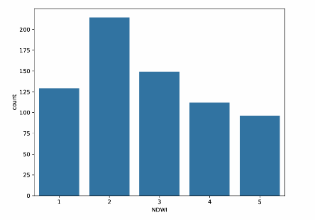
Figure 2. Count plot of NDWI in the training data

Histograms were then drawn for whether the landslide occurred in this dataset and for scenarios under different mv. It is not difficult to see that the occurrence times of landslides are different under the influence of different water content.

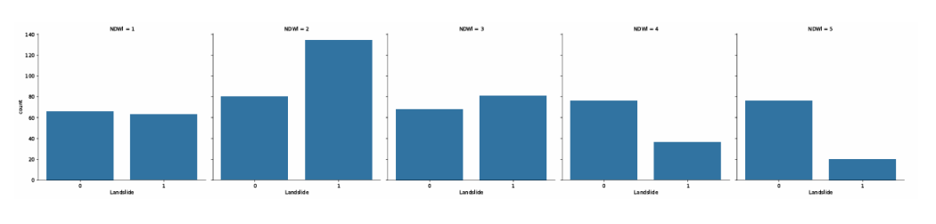
Figure 3. Count plot of Landslide occurrences by NDWI categories

In order to more intuitively study the relationship between soil moisture content and whether landslides occur, a probability graph was further drawn, that is, the probability of landslides occurring at different levels. From this probability graph, it is obvious that when the mv level is 2, the probability of a land- slide is the highest. This further illustrates that there is a strong link between soil moisture content and whether landslides occur.

4.2. Grades corresponding to different

Typical soils have a mv equal to 5% and become saturated when the mv reaches 40%. So based on the fact that the higher the mv the more prone to landslides and the analysis of the data set as above, we have made the following ratings for different mv, show in Table 1.

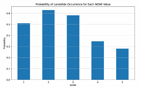
Figure 4. Probability of Landslide Occurrence for Each NDWI Value

Table 1. The grades for different mv

4.3. Parameter setting for Hidden

In this experiment, the Hidden Markov Model is used to predict whether a landslide is likely to occur in this region in the future. For this purpose, some values need to be defined. The hidden state space is set to ”0” and ”1”, indicating that landslides will occur and that landslides will not occur. This parameter setting is also consistent with ”0” and ”1” in the database. The observation space is ”1”, ”2”, ”3”, ”4”, and ”5”, representing the five different levels of mv. According to the database adopted in this study, the initial state distribution matrix, the state transition probabilities matrix, and the observation likelihoods matrix were calculated and defined. This completes all the parameters needed to train the model.

5. Experimental setup

We set the Pt equal to 19dBm, Gt and Gr equal to 2dBm, f equal to 0.43GHz, dug equal to 2m, dag equal to 10m, and η equal to 2. And we can get the Pr from the sensors. If we take measurements every other day and make predictions about them based on climate in a month, we will get a set of sequences of Pr shown as Table 2.

After training the model, we make predictions for 100 sets of data, of which 45 sets are known to have landslides and 55 sets are not.

Table 2. Set the Pr

6. Experiment results

Substituting the Pr into (9). we obtain a prediction of the spatial structure of the soil water content. After rating it, shown in Table 3, the landslide risk at this point in time is assessed as one of the factors influencing the random forest. And we get the predictions for the random forest, shown in Table 4. We can get a prediction accuracy of 91%.

Table 3. The mv level

Table 4. Prediction results

Based on the estimated changes in mv, the HMM model predicts at which point in the future the mv will be more likely to cause a landslide, shown in Table 4, in which 1 means that the mv in this case has a greater effect on the landslide, and 0 is a lesser effect.

We can get that after the 27th day this month, the mv is more likely to trigger land- slides. After considering several other influencing factors, we should pay more attention to these days and even warn the masses.

Table 5. Prediction of the degree of influence of mv on landslides

7. Conclusion

In general, this study first predicted the probability of landslides occurring in an area through the Random Forest machine learning model, and the prediction accuracy reached 91%. Then, according to the change factor of mv, the signal attenuation strength is analyzed and calculated, and the future change of mv in a region is predicted. This result is then put into the implicit Markov chain for risk assessment, and the time when landslides are most likely to occur in the future is obtained. This system is suitable for the high-frequency areas of landslides, which is convenient for people to prevent natural disasters and minimize the loss of human and material resources. But at the same time, some areas can be further studied and improved in the future, such as 3D modeling of the underground structure of the region, to more intuitively show the prediction results. In addition, studying different under- ground signal propagation to improve the ac- curacy of prediction.

Acknowledgement

Xinyu Zhou, Jingrui Wang and Linghao Tian contributed equally to this work and should be considered co-first authors.

References

[1]. Yashar Alimohammadlou, Asadallah Najafi, and Ali Yalcin. “Landslide process and impacts: A proposed classification method”. In: Catena 104 (2013), pp. 219–232.
[2]. Florent Avellaneda. “Efficient Inference of Optimal Decision Trees”. In: Proceedings of the AAAI Conference on Artificial Intelligence 34.04 (2020), pp. 3195– 3202.
[3]. Leo Breiman. “Random forests”. In: Ma- chine learning 45 (2001), pp. 5–32.
[4]. Matthieu Cord and Cunningham- Padraig. “Machine Learning Techniques for Multimedia”. In: Machine Learning Techniques for Multimedia (2008).
[5]. Matthew J. Cracknell and Anya M. Reading. “Geological Mapping Using Remote Sensing Data: A Comparison of Five Machine Learning Algorithms, Their Response to Variations in the Spatial Distribution of Training Data and the Use of Explicit Spatial Information”. In: Computers Geosciences 63 (2014), pp. 22–33.
[6]. FC Dai, Chin Fei Lee, and Y Yip Ngai. “Landslide risk assessment and management: an overview”. In: Engineering geology 64.1 (2002), pp. 65–87.
[7]. Xin Dong, Mehmet C Vuran, and Suat Irmak. “Autonomous precision agriculture through integration of wireless underground sensor networks with center pivot irrigation systems”. In: Ad Hoc Networks 11.7 (2013), pp. 1975–1987.
[8]. Stefano Luigi Gariano and Fausto Guzzetti. “Landslides in a changing cli- mate”. In: Earth-science reviews 162 (2016), pp. 227–252.
[9]. Vladimir Nasteski. “An Overview of the Supervised Machine Learning Methods”. In: HORIZONS.B 4 (2017), pp. 51–62.
[10]. Neil R Peplinski, Fawwaz T Ulaby, and Myron C Dobson. “Dielectric properties of soils in the 0.3-1.3-GHz range”. In: IEEE transactions on Geoscience and Remote sensing 33.3 (1995), pp. 803– 807.
[11]. Victor Rodriguez-Galiano et al. “Machine learning predictive models for mineral prospectivity: An evaluation of neu- ral networks, random forest, regression trees and support vector machines”. In: Ore Geology Reviews 71 (2015), pp. 804–818.
Cite this article
Zhou,X.;Wang,J.;Tian,L. (2025). Machine Learning for Prediction and Risk Assessment of Landslides. Applied and Computational Engineering,131,52-59.
Data availability
The datasets used and/or analyzed during the current study will be available from the authors upon reasonable request.
Disclaimer/Publisher's Note
The statements, opinions and data contained in all publications are solely those of the individual author(s) and contributor(s) and not of EWA Publishing and/or the editor(s). EWA Publishing and/or the editor(s) disclaim responsibility for any injury to people or property resulting from any ideas, methods, instructions or products referred to in the content.
About volume
Volume title: Proceedings of the 2nd International Conference on Machine Learning and Automation
© 2024 by the author(s). Licensee EWA Publishing, Oxford, UK. This article is an open access article distributed under the terms and
conditions of the Creative Commons Attribution (CC BY) license. Authors who
publish this series agree to the following terms:
1. Authors retain copyright and grant the series right of first publication with the work simultaneously licensed under a Creative Commons
Attribution License that allows others to share the work with an acknowledgment of the work's authorship and initial publication in this
series.
2. Authors are able to enter into separate, additional contractual arrangements for the non-exclusive distribution of the series's published
version of the work (e.g., post it to an institutional repository or publish it in a book), with an acknowledgment of its initial
publication in this series.
3. Authors are permitted and encouraged to post their work online (e.g., in institutional repositories or on their website) prior to and
during the submission process, as it can lead to productive exchanges, as well as earlier and greater citation of published work (See
Open access policy for details).