


1. Introduction
1.1. Relevance of the match predictions
From the 1960s onwards, there have been systematic efforts to forecast soccer match outcomes through statistical models [1], contrasting the prior forecasts that predominantly relied on expert knowledge. The escalating fascination with these models and forecasts can be primarily attributed to the growth of international sports betting market, which is worth several billion US dollars per year [2]
Forecasting a match mainly has two important stages. First, it is very important to collect as much useful information as possible about both teams. Right now, matches go through careful analysis and measurement. This is done especially by using automated methods. Groups can use this information to make tactical decisions. They can also find suitable players for possible future transfers.
In the context of match prediction, the performance strengths of the teams in particular can be estimated. Due to the limited information available before the match, the assessment of the performance of the two teams will always be subject to a certain degree of inaccuracy, but this can at least be minimized by optimizing the data used.
The next stage requires a model to predict the matches. This model takes data that already exists to make predictions. This means that the results can sometimes be guessed. Reep and Benjamin[3]have seen that luck plays an important role in the results of games. For example, teams with a higher market value do not always win matches. This unknown factor is a big part of what makes soccer very interesting. Therefore, the actual prediction consists of determining probabilities for all possible outcomes. There are various fundamental reasons why exact predictions are not possible [4]
Equilibrium between Fortune and Competence: Sport event results hinge on a combination of both luck and proficiency. Research shows that in very competitive events, luck plays a big role. This makes it hard for complicated models that focus on many details to do better than simple models. It means that no matter how advanced a model is, it is difficult to remove the effect of randomness completely.[5]
The Shortage and Instability of Data: Sports happenings are frequently plagued by a lack of information and instability. For example, when people try to predict the results of the NCAA men's basketball tournament, there are many challenges. One challenge is the many possible factors and sources of information. Another challenge is that players' performance can change a lot from one game to another. There is also not enough detailed history of data. All these things together make it hard to predict with models.[6]
Impact of Unforeseen Elements: The outcomes of sports events are influenced not only by what participants excel in but also by a variety of unforeseen elements. The unpredictable nature of these factors further complicates the prediction of results[7]
Concerning the Understanding of Models: Even with progress in machine learning and deep learning algorithms for predicting sports events, numerous models used in football science suffer from a lack of comprehensibility, hindering their efficient use.[8]Insufficient transparency may limit its applicability for analysts.
Complexity in Choosing and Assessing Models: Choosing and assessing models can be complicated. This is true for models that predict sports events. Picking these models needs many technical details. When you select a model, you have to check it, too. There are different ways to compute and use these models. Using different ways can cause wrong predictions. That means you might predict something that doesn't happen. It is important to choose the best, most efficient mix of models. This makes it more difficult.[9]
Obstacles in Data Processing and Feature Engineering: The stages of data purification, initial processing, and feature design are vital in creating efficient forecasting models.Nonetheless, the complexity of these procedures demands significant skill and experience.
Constraints in Model Generalization: Advanced models, too, can encounter their own generalization constraints. An illustration of this is the study on NBA game outcomes using decipherable machine learning, which revealed enhancements in Stacking model accuracy on the test set, yet the improvement was limited.[10]
First, the level of performance before must be good. Second, the model used must also be the best it can be. [11]
1.2. Machine learning in match prediction
Machine learning is special because it can easily learn from the growing amount of data in professional football. Kumar executed an evaluative comparison of different machine learning models focused on predicting soccer match outcomes.[12]After this, many more different models were brought in and tested very carefully. The main goal of these models is usually to predict the outcomes of matches. They do this by using data from history that we already know about. But it is important to say a few models make their guessing better. They do even more than before. They add new data taken during the games. This includes things like the condition of the field. It also includes how often each team has the ball. Another thing they include is how many shots they try to make.
Below is a concise summary of several models:
(1) Bayesian Networks [13]: This collection of statistical models brings together current knowledge. It also updates probability numbers with new information. This is done using Bayes' theorem. It helps to gain a deeper understanding of uncertainty. It also supports decision-making processes.
(2) Neural networks [14]: These computational frameworks, inspired by the human brain, decode data through connected points, or neurons, pinpointing patterns and making choices based on the received data.
(3) Random Forest [15]: A collective learning technique that enhances classification or regression precision by building several decision trees and deciding on their results. This system efficiently manages vast datasets and demonstrates resilience against noise and overfitting.
(4) K-Nearest-Neighbor [16]: To forecast a novel data point, it takes into account the K closest points in the feature space. The prediction of data point category or value relies on the classification categories (or regression values) of adjacent elements.
(5) Enhancing (XGBoost, CatBoost) [17]: An extensively employed framework for gradient amplification in machine learning contests. The system utilizes concurrent processing, aids in regularization, and successfully avoids overfitting. In performance metrics, XGBoost surpasses numerous other algorithms in computational efficiency.
(6) AdaBoost[18]: A repetitive algorithm merging various inferior categoryifiers (usually decision trees) through weighted voting enhances the precision of the model. Every cycle concentrates on incorrectly labeled samples from the last cycle, progressively improving the efficiency of the model.
(7) LightGBM[19]: An algorithm designed for gradient enhancement utilizing tree-based learning methods. Its design aims for distribution and efficiency while maintaining high accuracy.
1.3. Algorithm
1.3.1. Gaussian Regression
In Gaussian Process Regression, we believe a group of random things behaves like a big Gaussian distribution with many variables. If we know some observed variables called X1 and some unknown variables called X2, we can find out the possible distribution of X2 after seeing the data. The mean and covariance of the posterior distribution are given by:
\( Mean:{μ_{2|1}}={μ_{2}}+{Σ_{21}}Σ_{11}^{-1}({X_{1}}-{μ_{1}})Covariance:{Σ_{2|1}}={Σ_{22}}-{Σ_{21}}Σ_{11}^{-1}{Σ_{12}} \)
Where μ1, μ2 are the means of X1 and X2 respectively, and Σ11, Σ12, Σ21 , Σ22 are the covariance matrices.
1.3.2. Boosting
Boosting algorithms combine multiple weak learners into a strong learner. In XGBoost, the objective function is given by:
\( obj(θ)=\sum _{i=1}^{n} L({y_{i}},{\hat{y}_{i}})+\sum _{k=1}^{K} Ω({f_{k}}) \)
Where L is the loss function, y^i is the prediction, fk are the weak learners, and Ω is a regularization term.
1.3.3. AdaBoost
AdaBoost (Adaptive Boosting) adjusts the weights of the training samples based on the performance of the weak learners. The formula for the weight update is given by:
\( w_{i}^{(t+1)}=\frac{w_{i}^{(t)}exp(-{α_{t}}{y_{i}}{h_{t}}({x_{i}}))}{{Z_{t}}} \)
Where wi(t) is the weight of the i-th sample at iteration t, αt is the weight of the weak learner ht, yi is the true label, and Zt is a normalization factor.
1.3.4. Neural Networks
The formula for a neural network typically involves the forward propagation and backpropagation algorithms. In forward propagation, the input is passed through the network layer by layer to produce an output. The output of each neuron is given by:
a=σ(w⋅a+b)
Where σ is the activation function, w are the weights, a is the input (or the output of the previous layer), and b is the bias.
In backpropagation, the error is propagated backwards through the network to update the weights and biases. The weight update is given by:
\( {w_{ij}}={w_{ij}}-η\frac{∂E}{∂{w_{ij}}} \)
Where η is the learning rate, and E is the error function.
1.3.5. LightGBM
LightGBM is a gradient boosting framework based on decision trees. The formula for the prediction in LightGBM is similar to other gradient boosting algorithms, but with specific optimizations for handling large datasets and categorical features. The objective function in LightGBM is typically given by:
\( obj(θ)=\sum _{i=1}^{n} L({y_{i}},\hat{y}_{i}^{(t)})+\sum _{k=1}^{t} Ω({f_{k}})+constant terms \)
Where y^i(t) is the prediction at iteration t, fk are the decision trees, and Ω is a regularization term.
1.4. Simpson’s Paradox
Simpson's Paradox is a famous concept in the field of statistics ,which is firstly talked about by E.H. Simpson. This happened in the year 1951. When you look at data divided into different groups, you can find a specific pattern.But when you look at all the data together, this pattern might not be there. Sometimes it might even look opposite. This means, in a dataset, you could find a trend in separate groups. However, when you mix all the groups, this trend might vanish. Or, it could change to show the opposite direction.
Simpson's Paradox typically stems from a variety of reasons:
Weight Alignment: Groups with different sizes have different amounts of data. Also, these groups have different levels of importance. This creates a specific pattern. But this pattern does not match with what is happening now. It is a different pattern from the current ones.
Omitted Variables: There are some missing variables. We forgot to look at these variables. These parts that are missing can change the overall direction of the data.
The Simpson's Paradox impact on predicting sports outcomes appears mainly in these areas:
Model Prejudice: Sports prediction models may not manage or deal with combined data importance. They may ignore important factors. This can lead to incorrect model guesses. In sports events, looking at only the average performance of players can give a wrong idea. Not thinking about the small details of the game can make trouble. An example is the strength of the other team or where the game takes place. This can make people predict things that are not the same as the real situation.
Misleading Conclusions: A situation called Simpson's Paradox might make models wrong in what they say. Think about when you want to guess a team's chances to win; if you miss important things like the advantage of playing at home or away, you might make predictions that are the opposite of the actual game results.
(3) Increasing Complexity: Sports prediction systems need to handle information with more accuracy. They also need to deal with complex details. This helps avoid the effects of Simpson's Paradox. For example, more factors and control situations are needed. These help ensure the model shows the real game situation correctly.
(4) Study of a Case: A detailed case study helps us understand how Simpson's Paradox works in sports prediction. For instance, looking at shooting numbers of NBA players shows this. If we only look at how one player performs, we forget special conditions of the game. This might cause predictions that are not fair or true.
To summarize, the influence of Simpson's Paradox on sports forecasting models primarily manifests in biases, deceptive outcomes, and heightened intricacy.To successfully circumvent Simpson's Paradox effect, models predicting sports events should manage their data more precisely and take into account a broader range of factors and limitations [20][21]
1.5. Double chances
Within gambling, "Double Chance" refers to a betting strategy enabling gamblers to select simultaneously two distinct results.Such betting is frequently employed during football games, offering three potential results: victory for the home team, a tie, or triumph for the visiting team.Bettors can choose one of the following three combinations to place a bet:
Home win or draw (1 or X): If the match result is a home win or a draw, the bet is considered a win.
Draw or away win (X or 2): If the match result is a draw or an away win, the bet is considered a win.
Home win or away win (1 or 2): If the match result is a home win or an away win, the bet is considered a win.
2. Feature engineering
2.1. Dataset
The database encompasses comprehensive data (such as type of goals, ball holding, corner kicks, cross strikes, fouls, cards, etc...) about 25,000 games from EA Sports' FIFA series, featuring weekly summaries,spanning 2008 to 2016. It encompasses 10,000 players from the 11 European Countries with their lead championship and betting odds from up to 10 providers.[22]
2.2. Prediction of match outcome, goal difference,home and away,star member and exact match result
Various methods exist for forecasting a game's result. For the most basic form, only outcomes represented as win/draw/loss are taken into account.Foreseeing the disparity in goals is somewhat more precise.As previously noted, the precise alignment result is forecasted within the most informative variantconsidered by specifying the probabilities for all possible outcomes. More data is naturally required to predict the exact match result using data- driven models than when restricting to goal differences, as the number of possible exact match results is significantly larger than the number of possible goal differences. To make the outcome priciser ,home and away advantages, and the impact of star players are also pivotal factors that carry equal weight in predicting game results. Because the venue of the match can significantly influence the result due to factors like familiarity with the field, crowd support, and travel fatigue for the visiting team.And the presence and performance of key individuals can sway the game, as they often serve as decisive factors in critical moments.Recognizing the importance of these factors, we have focused on all the aspects. Our comprehensive analysis ensures that no stone is left unturned in our quest to forecast match results accurately. This multifaceted approach allows us to build robust predictive models that account for the dynamic nature of sports competitions.
2.3. Data Cleaning and Dimensionality Reduction
We conducted data cleansing and dimensionality diminution to guarantee data integrity and lay a dependable groundwork for future data examination and extraction.Here are the steps we took for data cleaning:
Auditing Data: We carefully looked at our data. We wanted to find any possible errors. There might be mistakes, missing parts, or strange data and so on. This step was very important. We needed to find specific problems in the data. These problems needed fixing.
Managing Missing Values: Missing data happens often. We needed to handle it. We could remove incomplete data. This might lead to losing some information. Or we could fill in the missing information. We did this after checking all parts of the data.
De-duplication: We needed to avoid mistakes. We did not want incorrect statistical results. So, we found and removed repeated data entries.
Treating Anomalies: Anomalies can change how accurate our model predictions are. We need to keep the data normal. This was done using statistical methods. One way is to use box plots.
Standardization of Format: We made data types the same. For example, date and number formats were made uniform. This was important for the whole dataset. If data formats are not consistent, it can cause wrong data reading and analysis.
Correcting Logical Errors: We used logic to find mistakes in our data. And then fix those logical mistakes. This was done to make sure these errors do not change our data analysis results.
To validate our data, we eliminated or amended any codes and values that failed to meet established standards.
To check if our data is correct, we removed or changed any codes and values that did not meet the rules we set. These actions were to make the data better. We did this by getting rid of extra noise, fixing mistakes, and making sure everything looks the same. This work helps to make data strong and ready for future use. Later, we did something to make the data smaller. We call this data dimensionality reduction. The main idea is to make the data size smaller. This helps to make our calculations simpler. It also makes our algorithms work better. These are our main steps for making data less complex:
Feature Selection: Important features were picked and removed from the list. This made our models simpler. It also made them faster to compute.
Principal Component Analysis (PCA) used PCA. It turned original high-dimensional features into smaller spaces step by step. This kept most of the data safe.
Linear Discriminant Analysis (LDA): We used LDA in our classification problems. Our goal was to reduce dimensions. This was done by making the gap bigger between different classes. It also made the distance smaller inside each class.
Making data smaller can really cut down the computational load on datasets that have many dimensions. These datasets need more processing power. At the same time, this way makes the model train and predict faster. It also reduces overfitting. It helps the model to work well with new data. Lastly, it makes it easier to understand the model.
2.4. Feature selection
2.4.1. Graphical analysis
Before starting to train the model, it is very important to arrange the data we have now. This data includes the time when the games happened. It also includes which teams played. It has the results of the games too. We need to check this data. This will make sure that everything works automatically.
Our team created probability density distributions and KDE charts to underscore the importance of the win-loss ratio between home and away games, evaluations by players, and their varied impacts on the results of matches.
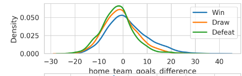
Figure 1. KDE chart of home team’s goals difference in the last 10 years
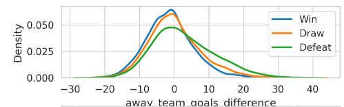
Figure 2. KDE chart of away team’s goals difference in the last 10 years
Each chart comes from checking a full 20000 elements in the dataset. We have a KDE chart. It shows how likely it is for goals to be different in the last ten games for both home and visiting teams. The result is clear. When the home team is in bad form, the away team has a higher chance to win. This happens if the home team's score is lower than the score they give up. But, if the home team is playing well, they have a bigger chance to win. This shows that with the advantage of playing at home, it is easier for the home team to win.
The second chart also proves this idea. The chart shows that when the away team is not in good form, the home team is still likely to win. Even when both teams are equal, at a score of zero, the home team has a good chance to win. The away team needs a high level of performance to win the game.
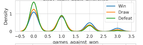
Figure 3. KDE chart of the chance of winning for home teams
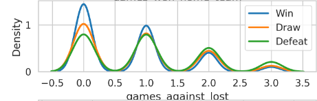
Figure 4. KDE chart of the chance of winning for away teams
After that, we looked at data about the last three games that the two teams played. The chance of winning for both home and away teams shows crossings in the Win and Defeat charts. This crossing suggests that there might be a fair effect on the game's results. But, you can see some differences.
Afterward, we checked the players' ratings. We looked at the players' average scores from teams playing at home or away. Next, we checked the chance for each team to win over different score times. It is clear that playing at home or away matters. When looking at the home team winning (blue curve) and away team winning (orange curve), their highest points in the probability charts are around a score of 75. This tells us that for both teams, an average player score of around 75 is an important number, no matter if they are playing at home or away. This peak at 75 might mean that, for most of the teams, a score of 75 is a normal and common score. This means the result of a game is not just about playing at home or away. It could mean that in this score range, the result is more affected by other things and not only if the game is home or away. This also shows that teams with a score around 75 are somewhat equally matched, making these game results harder to predict.
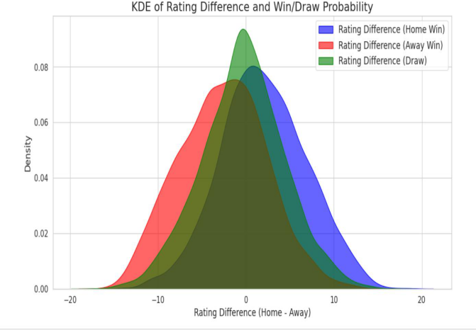
Figure 5. KDE of rating difference and win/Draw probability
The chart shows the probability for home and away teams in different based on different score changes. The chart shows a lot of score differences near 0, which means that the average score difference between home and away teams is small in most games. The sharp top of the green curve means that draws happen in specific situations, usually cases hen score differences are very small.
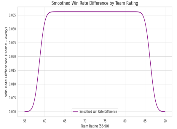
Figure 6. Smoothed win rate difference by team rating
Next, we used the Kernel Density Estimation (KDE) to balance the different win rates between the home and away teams. After adding the win rates from both teams and measuring the difference, the middle part of the graph shows teams' scores between 60 and 85. The win rate difference between home and away teams stays nearly the same, around 0.035. This means the home team has a steady advantage in these score situations, which goes against the idea that the home advantage gets smaller with higher scores. The drop in numbers below 60 and above 85, which are extreme situations within the 20,000 data points, further proves the home advantage is similar across parts.
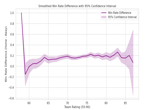
Figure 7. Smoothed win rate difference with 95% confidence interval
By checking the win rate differences between home and away teams, we explored this difference across different score ranges (from 55 to 90) and figured out the 95% confidence level for each score range. The big confidence range means there is certainty about the win rate difference at different scores. A big confidence range in one score range means fewer cases and less sure estimates of the win rate difference. A small confidence range gives more sure estimates within that score range. Big changes and big confidence ranges happen in areas with low scores (below 60) and high scores (above 85), proving fewer cases in these ranges make big confidence ranges and more uncertainty. The big confidence range near 85 means not enough data in this area, leading to less correct predictions.
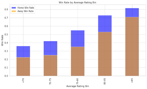
Figure 8. win rate difference between home and away by Average Rating Bin
Next, we organized our data into sections with home and away ratings. This is our final data chart. We see that the win rate difference between home and away is stable. This is true for both high scores and low scores. Only when scores are more than 85, the difference change. The reason is like we said before. There are fewer samples for scores greater than 85. Even if fewer samples cause the difference, the win rate of the home team is still higher than the away team. This further proves our guess from another angle.
2.4.2. Statistical Tests
Table 1. Chi-square of different rating groups
rating_bin | chi2 | p_value | degrees of freedom | |
0 | 70-75 | 28.716803 | 5.810660e-07 | 2 |
1 | 75-80 | 33.797279 | 4.581568e-08 | 2 |
2 | 80-85 | 30.735210 | 2.118039e-07 | 2 |
3 | <70 | 2.149495 | 3.413840e-01 | 2 |
4 | >85 | 7.650000 | 2.181844e-02 | 2 |
Our process started by dividing the data into specific rating groups. Then, we performed the Chi-square test on these groups. We found an interesting trend. For people aged 70 to 85, the impact of factors from home and away was important. This is because teams in this group are quite similar in skill. So, outside factors like home crowd support and being familiar with the playing surface affect the results more. On the other hand, in the group with a rating over 85, top teams compete hard. Home advantage still matters here. Even small outside factors can change the outcomes of important games. However, in the score group under 70, the effect of the home versus away elements was less.
At first, we thought that the home advantage would be more noticeable with low scores. We believed its impact would get smaller as the average score increased. The 75-80 score range seemed to be a significant high. But then we discovered it was a Simpson's Paradox. This happened due to having too few numbers in our data set. So, we increased the amount of data to 20,000.And stated below are the new result.
Table 2. Chi-square of different rating groups after data extension
| rating_bin | chi2 | p_value | degrees_of_freedom |
0 | 70-75 | 407.826933 | 2.763801e-89 | 2 |
1 | <70 | 214.919618 | 2.141894e-47 | 2 |
2 | 75-80 | 264.186021 | 4.292738e-58 | 2 |
3 | 80-85 | 60.928070 | 5.883527e-14 | 2 |
4 | >85 | 9.310345 | 9.512273e-03 | 2 |
2.4.3. Model Results
Table 3. Pseudo-r-squared outcome of home and away team average rating
| coef | std err | z | P>|z| | [0.025 | 0.975] |
home _ team _ avg _ rating | 0.7214 | 0.067 | 10.841 | 0.000 | 0.591 | 0.852 |
away _ team _ avg _ rating | -0.8036 | 0.070 | -11.525 | 0.000 | -0.940 | -0.667 |
interaction | -0.0059 | 0.069 | -0.086 | 0.932 | -0.141 | 0.129 |
We used ratings from both home and away teams as main factors. The pseudo-R-squared measure shows the model accounts for about 11.22% of the change in the target variable. This is a reasonable amount for classification models and suggests some explanatory power. Compared to the null model, the Log-Likelihood model did better. We found that for every standard increase in the home team's rating, the log odds of winning rose by 0.7214, a significant finding (p < 0.05). This shows a better home team is more likely to win if other factors stay the same. Raising the away team's rating, however, lowers the home team's chance of winning by 0.8036, also statistically meaningful (p < 0.05). This indicates a higher chance of the away team winning. Interestingly, the connection between home and away team ratings was weak. There was a small coefficient and a p-value over 0.05. This tells us that the total impact of both teams' ratings doesn't majorly change results, stressing their separate effects.
Table 4. MNLogit Regression result
label_numeric=1 | coef | stderr | z | P>|z| | [0.025 | 0.975] |
home_team_avg_rating | 0.0973 | 0.004 | 21.668 | 0.000 | 0.089 | 0.106 |
away_team_avg_rating | -0.0993 | 0.005 | -22.027 | 0.000 | -0.108 | -0.090 |
interaction | 0.0001 | 6.11e-05 | 2.035 | 0.042 | 4.56e-06 | 0.000 |
label_numeric=2 | coef | stderr | z | P>|z| | [0.025 | 0.975] |
home_team_avg_rating | -0.0989 | 0.005 | -20.326 | 0.000 | -0.108 | -0.089 |
away_team_avg_rating | 0.0998 | 0.005 | 19.776 | 0.000 | 0.090 | 0.110 |
interaction | -1.656e-05 | 6.7e-05 | -0.247 | 0.805 | 0.000 | 0.000 |
We later expanded our data to 20000 entries. After cleaning, we worked with 18,318 entries. We used Multinomial Logistic Regression and MNLogit, for analysis. We took a draw as a baseline. In the interaction terms, the impact of the away team compared to a draw was not significant. But the impact of the home team winning compared to a draw was significant. It was very small, only 0.0001. This also shows from another angle that when both home and away team scores go up, the home team gains a slight winning advantage. This also shows the home advantage from another view.
Finally, for elite players with at least 85 points, their presence or absence affects results greatly. But strangely, key home players increase the chance of away team wins, against common sense. We ruled out sample size issues first. Then, we found strong multicollinearity between home and away scores, which might explain this strange result.
2.5. Final feature set
Following numerous selections in feature engineering and experimental evaluations, we ultimately identified this collection of features:
Variation in goals between home and away teams
Victory in Games with the Home&Away squad
Competitions featuring Won & Lost
The average rating for the home and away teams
benefit at home
Variation in team scores
The renowned home and away player
The features showed important ability to predict and explain in our model. This makes a strong base for guessing which team will win a football match.
3. Models for Match Prediction
3.1. Model selection
A range of algorithms were evaluated to pinpoint the most effective model, with their precision assessed.
• Gaussian regression
• Neural networks
• Random Forest
• K-Nearest-Neighbor
• Boosting (XGBoost, CatBoost)
• AdaBoost
• LightGBM
3.2. Comparison of models
Table 5. Comparison of models
| Precision | recall | fl-score | support | accuracy | |
Random Forrest | 0.46 | 0.5 | 0.46 | 3664 | 0.503 | |
Ada Boost | 0.39 | 0.53 | 0.44. | 3664 | 0.528 | |
GaussianNB | 0.47 | 0.53 | 0.44 | 3664 | 0.527 | |
Kneighbors | 0.46 | 0.48 | 0.46 | 3664 | 0.476 | |
Logistic Regression | 0.47 | 0.49 | 0.47 | 3664 | 0.491 | |
XGB | 0.45 | 0.52 | 0.44 | 3664 | 0.523 | |
LGBM | 0.51 | 0.53 | 0.44 | 3664 | 0.526 | |
State above are the outcomes of our test in the single chance circunstance,in the chart,0 represents lose game,1 represents draw games,2 represents win games, we make out an average accuracy score,and among all the model, LGBM Classifier and Ada boost performed the better ,with the accuary of 52.6% and 52.8%
3.2.1. Double chances result
Table 6. models’ double chances result
| Precision | recall | fl-score | support | accuracy | |
Random Forrest | 0.46 | 0.5 | 0.46 | 3664 | 0.503 | |
GaussianNB | 0.47 | 0.48 | 0.48 | 3664 | 0.484 | |
LGBM | 0.46 | 0.51 | 0.46 | 3664 | 0.778 |
We then tested the accuracy of every model in the double chances situation,and we find out that all the performance of model have a great improvement,and the ada boost model performed the best with an accuracy of 78%
3.2.2. Result deleted draw situation
After the test we did ,we found out that the prediction accuracy of draw game is obviosly low than other two ,so we did anthor model only predict win and draw game ,and it turns out that the accuracy can be higher that before ,which is 70.4%
4. Simulation Betting
4.1. Method
We performed a betting simulation activity. We used all 3,664 pieces of data for placing bets. In this data, only 275 instances had a difference greater than 0.05 between the predicted chances and the chances predicted by our model. This activity ended with a profit of 11,279 yuan. This is a profit rate of 3%. To prevent any logical errors and prove our betting plan is accurate, we picked the first five betting records to check. This was to make sure our prediction method is trustworthy.
4.2. Model Evaluation
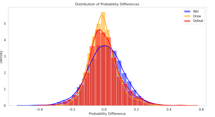

Figure 9. distribution of probability difference between our model and market’s model
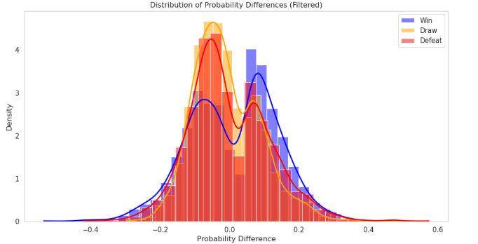

Figure 10. distribution of probability difference of win chances between our model and market’s model
In our study, we compared our prediction models with those from betting companies. The first picture shows the difference between the chances predicted by our model and the chances that come from the betting markets. Afterward, we did a special study to find and look at data points that might allow for arbitrage. We calculated the average and differences of these situations. We found arbitrage chances by looking at the gap between the win chances from our model and those from the bookmakers' odds. We used 0.05 as the measure to think a data point could have an arbitrage chance. After checking 275 data points, we saw the difference was small in both cases. This shows our prediction results are very similar to those of the betting companies. This similarity helps prove our model is reliable and works well, supporting its truth.
5. Discussion
5.1. Problem
This study has found some results in building a model to predict the win rate of football matches. But there are still some weaknesses. First, because there is not enough time and database resources, the model's feature engineering has limited factors. These factors include things like public opinion analysis, feelings analysis, and economic content analysis. These limited factors have made the model less complete and less accurate. Second, the model was tested and validated. However, the process might not have checked all scenarios and changes. This means the model's stability and reliability in real-life use need more testing. Lastly, the models have not done well when predicting draws. But in the samples, draws happen quite a bit. Even after using SMOTE sampling process, we saw something interesting. When we looked at the graph that shows the score difference between home and away teams, we noticed something. The curve for draws was very sharp. This means that the early prediction conditions for draws were too strict.
5.2. Future plan
For future research, several directions can be explored:
• Incorporating venue conditions, weather, public opinion, and economic factors to enhance model accuracy and granularity.
• Expanding the dataset to include other football leagues to improve model robustness and comprehensiveness.
• Searching for additional data and methods to refine the model's prediction of draws.
Acknowledgement
Eryi Wang and Xinyi Yin contributed equally to this work and should be considered co-first authors.
References
[1]. ubitzky, W., Lopes, P., Davis, J. et al. The Open International Soccer Database for machine learning. Mach Learn, 2019 108, 9-28. https://doi.org/10.1007/s10994-018-5726-0
[2]. Etuk, R., Xu, T., Abarbanel, B., Potenza, M. N., & Kraus, S. W. Sports betting around the world: A systematic review. Journal of Behavioral Addictions 2022, 11,3,689-715. https://doi.org/10.1556/2006.2022.00064
[3]. Goes, F. R., Meerhoff, L. A., Bueno, M. J. O., Rodrigues, D. M., Moura, F. A., Brink, M. S. ElferinkGemser, M.T., Knobbe, A.J., Cunha, S.A., Torres, R.S., Lemmink, K. A. P. M., Unlocking the potential of big data to support tactical performance analysis in professional soccer: A systematic review. European Journal of Sport Science 2020, 21(4), 481-496.
[4]. Heuer, A. Der perfekte Tipp: Statistik des Fussballspiels, Wiley-VCH 2012, Weinheim.
[5]. Raquel Y.S. Aoki, Renato M. Assuncao, and Pedro O.S. Vaz de Melo. 2017. Luck is Hard to Beat: The Difficulty of Sports Prediction. In Proceedings of the 23rd ACM SIGKDD International Conference on Knowledge Discovery and Data Mining (KDD '17). Association for Computing Machinery, New York, NY, USA, 1367–1376. https://doi.org/10.1145/3097983.3098045
[6]. Yuan, L., Liu, A., Yeh, A., Kaufman, A., Reece, A., Bull, P., Franks, A., Wang, S., Illushin, D. & Bornn, L. (2015). A mixture-of-modelers approach to forecasting NCAA tournament outcomes. Journal of Quantitative Analysis in Sports, 11(1), 13-27. https://doi.org/10.1515/jqas-2014-0056
[7]. Wang, Junjian, [Retracted] Mining and Prediction of Large Sport Tournament Data Based on Bayesian Network Models for Online Data, Wireless Communications and Mobile Computing, 2022, 1211015, 8 pages, 2022. https://doi.org/10.1155/2022/1211015
[8]. Zhang Shaoliang, Yang Banban, Chen Lei. Research on the Prediction Model of Chinese Football Super League Driven by Ensemble Learning. Proceedings of the 13th National Conference on Sports Science - Special Reports (Sports Statistics Section), 2023.
[9]. Miao, Zhongli, Hu, Youhong, [Retracted] Research and Analysis of Combination Forecasting Model in Sports Competition, Journal of Sensors, 2022, 5945599, 10 pages, 2022. https://doi.org/10.1155/2022/5945599
[10]. Sun Chunjie. Analysis and Prediction of NBA Game Results Based on Explainable Machine Learning [D]. Jiangsu Province: Soochow University, 2023. DOI: 10.27351/d.cnki.gszhu.2023.001979.
[11]. Fischer M, Heuer A. Match predictions in soccer: Machine learning vs. Poisson approaches[J]. arXiv preprint arXiv:2408.08331, 2024.
[12]. Kumar, G. Machine Learning for Soccer Analytics, PhD Thesis 2013, 10.13140/RG.2.1.4628.3761
[13]. Constantinou, A.C. Dolores: a model that predicts football match outcomes from all over the world. Mach Learn 2019, 108, 49-75. https://doi.org/10.1007/s10994-018-5703-7
[14]. Mendes-Neves, T., Mendes-Moreira, J. Comparing State-of-the-Art Neural Network Ensemble Methods in Soccer Predictions. In: Helic, D., Leitner, G., Stettinger, M., Felfernig, A., Raś, Z.W. (eds) Foundations of Intelligent Systems 2020. ISMIS 2020. Lecture Notes in Computer Science(), vol 12117. Springer, Cham. https://doi.org/10.1007/978-3-030-59491-6_13
[15]. Stübinger, J.; Mangold, B.; Knoll J. Machine Learning in Football Betting: Prediction of Match Results Based on Player Characteristics. Appl. Sci. 2022, 10, 46, https://doi.org/10.3390/app10010046
[16]. Berrar, D., Lopes, P., Dubitzky, W. Incorporating Domain Knowledge in Machine Learning For Soccer Outcome Prediction. Mach Learn 2018, 108, 97-126. https://doi.org/10.1007/s10994-018- 5747-8
[17]. Yeung, C; Bunker, R; Umemoto R.; Fujiii, K. Evaluating Soccer Match Prediction Models: A Deep Learning Approach and Feature Optimization for Gradient-Boosted Trees, arXiv 2023, https://doi.org/10.48550/arXiv.2309.14807
[18]. B. Ji and J. Li, "NBA All-Star Lineup Prediction Based on Neural Networks," 2013 International Conference on Information Science and Cloud Computing Companion, Guangzhou, China, 2013, pp. 864-869, doi: 10.1109/ISCC-C.2013.92.
[19]. Wenyu Liu, Xi Xu, Yongqiang Cui, and Di Bai. 2024. In Proceedings of the 2024 International Academic Conference on Edge Computing, Parallel and Distributed Computing (ECPDC '24). Association for Computing Machinery, New York, NY, USA, 90–95. https://doi.org/10.1145/3677404.3677420
[20]. Mazaheri B, Jain S, Cook M, et al. Distribution Re-weighting and Voting Paradoxes[J]. arXiv preprint arXiv:2311.06840, 2023.
[21]. Hovhannisyan A, Allahverdyan A E. Resolution of Simpson's paradox via the common cause principle[J]. arXiv preprint arXiv:2403.00957, 2024.
[22]. Hugo Mathien.2016.European Soccer Database[Data set].EA Sports' FIFA games.
Cite this article
Wang,E.;Yin,X.;Li,Y.;Wang,T. (2025). Sports Betting: An Application of Machine Learning to the Game Prediction. Applied and Computational Engineering,132,104-118.
Data availability
The datasets used and/or analyzed during the current study will be available from the authors upon reasonable request.
Disclaimer/Publisher's Note
The statements, opinions and data contained in all publications are solely those of the individual author(s) and contributor(s) and not of EWA Publishing and/or the editor(s). EWA Publishing and/or the editor(s) disclaim responsibility for any injury to people or property resulting from any ideas, methods, instructions or products referred to in the content.
About volume
Volume title: Proceedings of the 2nd International Conference on Machine Learning and Automation
© 2024 by the author(s). Licensee EWA Publishing, Oxford, UK. This article is an open access article distributed under the terms and
conditions of the Creative Commons Attribution (CC BY) license. Authors who
publish this series agree to the following terms:
1. Authors retain copyright and grant the series right of first publication with the work simultaneously licensed under a Creative Commons
Attribution License that allows others to share the work with an acknowledgment of the work's authorship and initial publication in this
series.
2. Authors are able to enter into separate, additional contractual arrangements for the non-exclusive distribution of the series's published
version of the work (e.g., post it to an institutional repository or publish it in a book), with an acknowledgment of its initial
publication in this series.
3. Authors are permitted and encouraged to post their work online (e.g., in institutional repositories or on their website) prior to and
during the submission process, as it can lead to productive exchanges, as well as earlier and greater citation of published work (See
Open access policy for details).
References
[1]. ubitzky, W., Lopes, P., Davis, J. et al. The Open International Soccer Database for machine learning. Mach Learn, 2019 108, 9-28. https://doi.org/10.1007/s10994-018-5726-0
[2]. Etuk, R., Xu, T., Abarbanel, B., Potenza, M. N., & Kraus, S. W. Sports betting around the world: A systematic review. Journal of Behavioral Addictions 2022, 11,3,689-715. https://doi.org/10.1556/2006.2022.00064
[3]. Goes, F. R., Meerhoff, L. A., Bueno, M. J. O., Rodrigues, D. M., Moura, F. A., Brink, M. S. ElferinkGemser, M.T., Knobbe, A.J., Cunha, S.A., Torres, R.S., Lemmink, K. A. P. M., Unlocking the potential of big data to support tactical performance analysis in professional soccer: A systematic review. European Journal of Sport Science 2020, 21(4), 481-496.
[4]. Heuer, A. Der perfekte Tipp: Statistik des Fussballspiels, Wiley-VCH 2012, Weinheim.
[5]. Raquel Y.S. Aoki, Renato M. Assuncao, and Pedro O.S. Vaz de Melo. 2017. Luck is Hard to Beat: The Difficulty of Sports Prediction. In Proceedings of the 23rd ACM SIGKDD International Conference on Knowledge Discovery and Data Mining (KDD '17). Association for Computing Machinery, New York, NY, USA, 1367–1376. https://doi.org/10.1145/3097983.3098045
[6]. Yuan, L., Liu, A., Yeh, A., Kaufman, A., Reece, A., Bull, P., Franks, A., Wang, S., Illushin, D. & Bornn, L. (2015). A mixture-of-modelers approach to forecasting NCAA tournament outcomes. Journal of Quantitative Analysis in Sports, 11(1), 13-27. https://doi.org/10.1515/jqas-2014-0056
[7]. Wang, Junjian, [Retracted] Mining and Prediction of Large Sport Tournament Data Based on Bayesian Network Models for Online Data, Wireless Communications and Mobile Computing, 2022, 1211015, 8 pages, 2022. https://doi.org/10.1155/2022/1211015
[8]. Zhang Shaoliang, Yang Banban, Chen Lei. Research on the Prediction Model of Chinese Football Super League Driven by Ensemble Learning. Proceedings of the 13th National Conference on Sports Science - Special Reports (Sports Statistics Section), 2023.
[9]. Miao, Zhongli, Hu, Youhong, [Retracted] Research and Analysis of Combination Forecasting Model in Sports Competition, Journal of Sensors, 2022, 5945599, 10 pages, 2022. https://doi.org/10.1155/2022/5945599
[10]. Sun Chunjie. Analysis and Prediction of NBA Game Results Based on Explainable Machine Learning [D]. Jiangsu Province: Soochow University, 2023. DOI: 10.27351/d.cnki.gszhu.2023.001979.
[11]. Fischer M, Heuer A. Match predictions in soccer: Machine learning vs. Poisson approaches[J]. arXiv preprint arXiv:2408.08331, 2024.
[12]. Kumar, G. Machine Learning for Soccer Analytics, PhD Thesis 2013, 10.13140/RG.2.1.4628.3761
[13]. Constantinou, A.C. Dolores: a model that predicts football match outcomes from all over the world. Mach Learn 2019, 108, 49-75. https://doi.org/10.1007/s10994-018-5703-7
[14]. Mendes-Neves, T., Mendes-Moreira, J. Comparing State-of-the-Art Neural Network Ensemble Methods in Soccer Predictions. In: Helic, D., Leitner, G., Stettinger, M., Felfernig, A., Raś, Z.W. (eds) Foundations of Intelligent Systems 2020. ISMIS 2020. Lecture Notes in Computer Science(), vol 12117. Springer, Cham. https://doi.org/10.1007/978-3-030-59491-6_13
[15]. Stübinger, J.; Mangold, B.; Knoll J. Machine Learning in Football Betting: Prediction of Match Results Based on Player Characteristics. Appl. Sci. 2022, 10, 46, https://doi.org/10.3390/app10010046
[16]. Berrar, D., Lopes, P., Dubitzky, W. Incorporating Domain Knowledge in Machine Learning For Soccer Outcome Prediction. Mach Learn 2018, 108, 97-126. https://doi.org/10.1007/s10994-018- 5747-8
[17]. Yeung, C; Bunker, R; Umemoto R.; Fujiii, K. Evaluating Soccer Match Prediction Models: A Deep Learning Approach and Feature Optimization for Gradient-Boosted Trees, arXiv 2023, https://doi.org/10.48550/arXiv.2309.14807
[18]. B. Ji and J. Li, "NBA All-Star Lineup Prediction Based on Neural Networks," 2013 International Conference on Information Science and Cloud Computing Companion, Guangzhou, China, 2013, pp. 864-869, doi: 10.1109/ISCC-C.2013.92.
[19]. Wenyu Liu, Xi Xu, Yongqiang Cui, and Di Bai. 2024. In Proceedings of the 2024 International Academic Conference on Edge Computing, Parallel and Distributed Computing (ECPDC '24). Association for Computing Machinery, New York, NY, USA, 90–95. https://doi.org/10.1145/3677404.3677420
[20]. Mazaheri B, Jain S, Cook M, et al. Distribution Re-weighting and Voting Paradoxes[J]. arXiv preprint arXiv:2311.06840, 2023.
[21]. Hovhannisyan A, Allahverdyan A E. Resolution of Simpson's paradox via the common cause principle[J]. arXiv preprint arXiv:2403.00957, 2024.
[22]. Hugo Mathien.2016.European Soccer Database[Data set].EA Sports' FIFA games.