1. Introduction

The increasing demand for remote sensing data has led to an exponential growth in the volume of MS and multitemporal image datasets. These datasets are essential for applications such as disaster monitoring, environmental change detection, and urban planning, where accurate and quick analysis of changes over time is critical. However, the large data sizes generated by MS imaging systems, particularly from spaceborne satellites, present significant challenges for storage, transmission, and processing. For instance, the Sentinel-2 satellite system produces terabytes of data every few days, resulting in rapidly growing archives expected to surpass 100 petabytes by 2030 [1]. Addressing these challenges requires advanced compression techniques that balance efficiency with image quality.

Previous studies on MS and hyperspectral (HS) image compression have explored traditional methods such as wavelet-based transforms like JPEG2000 [2], predictive approaches like Least Mean Squares (LMS) and Recursive Least Squares (RLS) [3][4], and standards like CCSDS 123.0-B-2 [5]. Recently, deep learning techniques, including convolutional neural networks (CNNs), GANs, and autoencoders, have shown significant advancements [6][7]. For example, GAN-based methods like Agustsson et al. [8] achieved high compression at low bit rates, while CNN frameworks such as Valsesia and Magli [9] provided efficient reconstruction aligned with standard compression protocols. These methods emphasize the growing role of deep learning in addressing the challenges of large-scale MS data compression.

Traditional MS image compression methods like JPEG2000 utilize spatial and spectral redundancies within individual images but often ignore temporal correlations between images captured at different times over the same region. Leveraging these correlations can improve compression performance. Advanced deep learning models, like Pix2Pix [10] and MultiTempGAN [11], use GANs to achieve high compression ratios for multitemporal MS data. Specifically, MultiTempGAN uses a GAN model to estimate the target image based on a given reference image. However, these models may face limitations due to large parameter sizes and high computational demands. Q-MultiTempGAN addresses these issues by reducing model size using fewer bits for representing weights, and maintains performance while enabling deployment in resource-constrained environments like satellite systems.

2. Datasets and Image Preparation

The performance of Q-MultiTempGAN was evaluated on the same three datasets used in the MultiTempGAN paper, each consisting of a single Sentinel-2 satellite MS image pair from different regions of Turkey captured across various time periods. These large MS image pairs were first up-sampled to 10 m spatial resolution [12] using the SNAP toolbox [13] and then divided into 441 non-overlapping patch pairs. Each patch pair consists of a reference patch (earlier-sensed image) and a target patch (later-sensed image) and every patch in the pair has dimensions of 512 × 512 × 12, which means that each patch pair has dimensions of 1024 × 512 × 12, where the left half represents the target image and the right half represents the reference image. Since visualizing all 12 channels of MS patch pairs is impractical, every three channels are combined to form a 1024 × 512 × 3 RGB representation, resulting in each MS image patch pair being represented as four RGB pairs. The goal of MultiTempGAN was to train a model using these patch pairs to predict the target image patch using the reference image patch. Q-MultiTempGAN achieves the same purpose while utilizing quantization techniques to compress the model and reduce computational requirements. Detailed dataset specifications are provided in Table 1.

Table 1: Details of the datasets used in the proposed model.

3. Proposed Model: Q-MultipTempGAN

As the main aim of Q-MultiTempGAN was to propose a more lightweight and still reasonably accurate model using GAN just like what the base study of this paper, MultiTempGAN, did for compression of multitemporal MS images by evaluating the performance metrics of approaches like U-Net [14], LinkNet [15], and ResNet [16] and proposing a customized version of Pix2Pix with lower complexity by reducing the number of convolutional layers and capability of accepting input images with 12 channels, in this study several quantization approaches were implemented, the observed results were stored and taken into comparison to choose the most appropriate approach over the same datasets that were used in MultiTempGAN. The datasets and the details that were helpful in choosing the best quantization approach are mentioned in sections 2 and 4, respectively.

Figure 1 illustrates the structure of the proposed Q-MultiTempGAN model, designed to address the limitations of MultiTempGAN. The generator, discriminator, and quantization processes are detailed, showcasing a framework that balances efficiency and performance. The model employs various quantization strategies, including uniform quantization and mixed precision quantization, applied at different bit-width configurations to significantly reduce memory and computational requirements while maintaining high image quality. Experiments on Sentinel-2 multitemporal MS datasets demonstrate that Q-MultiTempGAN achieves comparable SNR and bpp performance to state-of-the-art models, while enabling efficient deployment for large-scale remote sensing applications. This highlights the potential of advanced quantization methods as key tools for optimizing deep learning-based compression.

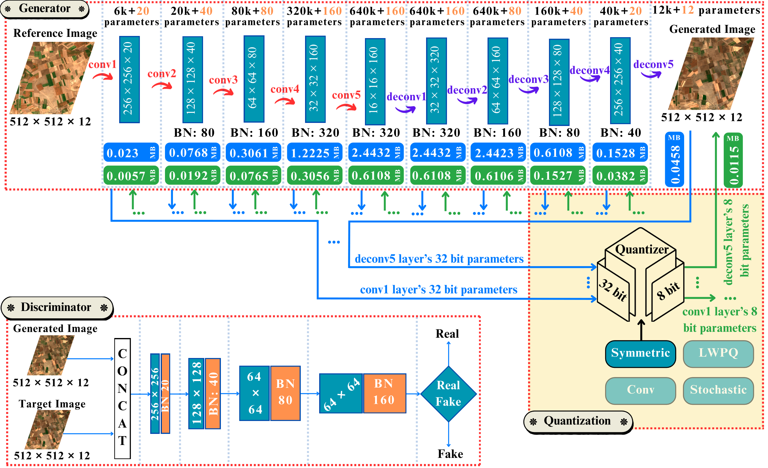
Figure 1: The generator structure is shown at the top, with convolutional layers (conv1–conv5) and deconvolution layers (deconv1–deconv5). Batch Normalization layers (BN) are highlighted below, with the number of parameters above each layer and biases in orange. Storage requirements for 32-bit parameters are shown in blue boxes, and post-quantization storage (8-bit symmetric quantization) in green. The discriminator structure is shown at the bottom left, where CONCAT denotes concatenation, and the final layer outputs real/fake probabilities. The quantization process at the bottom right includes Symmetric, Layer-Wise Precision (LWPQ), selective convolutional layer (Conv), and Stochastic Quantization, detailing operations for parameter selection.

4. Quantization Approaches

In this study, after retraining the original MultiTempGAN model and saving its final checkpoint, various post-training quantization approaches were investigated, and the model parameters were quantized to different bit rates using each method. The quantization techniques were categorized into two main groups: Mixed-Precision Quantization and Uniform Quantization. Key metrics, including SNR, bpp and Laplacian Mean Square Error (LMSE), were evaluated and compared against those of the original MultiTempGAN. Based on these comparisons, the most suitable quantization approach and bit rate were determined. Detailed results and metrics for both MultiTempGAN and Q-MultiTempGAN, along with the specifics of each quantization approach, are presented in the following subsections.

The original MultiTempGAN model includes 2,560,252 generator parameters, distributed across various layers categorized into the encoder (conv1 to conv5), decoder (deconv1 to deconv5), and Batch Normalization (BN). During quantization, the total number of generator parameters remains unchanged, but each parameter is stored using fewer bits.

All quantization approaches introduce additional parameters, referred to as side information, such as scales, zero points, and related values. These side information parameters are essential for reconstructing the original values during dequantization. Although small, their presence slightly impacts bpp. As defined in Equation 1, bpp is calculated as:

\( bpp=\frac{\ \ \ quantized\_parameters × bit\_precision + \ \ \ side\_information × 32}{\ \ \ pixels × \ \ \ images} \) (1)

Here, #quantized_parameters represents the total number of generator parameters that are quantized using a specific approach. Each of these parameters is stored with a precision defined by #bit_precision, which indicates the number of bits used to represent each quantized parameter. #side_information refers to additional parameters, such as scales and zero points, required for dequantization, with each side information parameter stored using 32 bits. #pixels represents the total number of pixels in a single MS image, calculated as 512 × 512 × 12, and #images refers to the total number of images (patches) in the dataset, which is 441. The effect of side information on bpp depends on the quantization method and is elaborated upon in the following subsections.

During the implementation phase, quantization process was performed using the following bit widths: 2, 4, 6, 8, 16, and 32. Quantizing to 32 bits provided a baseline comparison with the original model to assess the impact of quantization. Notably, 6-bit and 8-bit quantization offered the best balance between compression and accuracy, with key metrics such as SNR, bpp and LMSE closely approximating those of the original model. For simplicity, only the results for 6-bit and 8-bit quantization and the approaches with the best performance are included in Table 2 which presents the detailed results.

This study utilized three distinct datasets, and performance metrics were averaged across them. For example, the SNR for the original MultiTempGAN model was calculated as 27.87, 26.43, and 24.72 for MSI Pair-1, MSI Pair-2, and MSI Pair-3, respectively, that result in an average of 26.34, as reported in Table 2. This averaging approach was also consistently applied to LMSE, and across all evaluated models, including ResNet, LinkNet, and others, to ensure a comprehensive comparison.

4.1. Uniform Quantization

Uniform quantization involves quantizing all model parameters or weights to the same fixed bit width throughout the model [17]. This category of quantization is relatively simple to implement and is highly hardware-friendly due to its minimal customization requirements. However, it may have a negative impact in layers that are more sensitive to precision loss. In this study, the following uniform quantization methods were evaluated: Quantizing All Weights, Linear Quantization, Symmetric Quantization, Asymmetric Quantization, Stochastic Quantization, and Integer Quantization.

For clarity, Linear Quantization divides the range uniformly into levels, making it simple and fast to implement [17][18]. Fixed-Point Quantization converts floating-point numbers to fixed-point representation, optimizing it for hardware acceleration [17][19]. Symmetric Quantization uses quantization levels centered around zero, reducing computational overhead and improving model compatibility [17]. Asymmetric Quantization accommodates data distributions with offset means, better handling skewed data and achieving higher accuracy for certain tasks [17]. Lastly, Stochastic Quantization introduces randomness to avoid artifacts, rounding weights probabilistically to improve generalization [17].

Among the uniform quantization approaches evaluated in this study, Stochastic Quantization and Symmetric Quantization using 8-bit precision showed the best performance across key metrics such as SNR and bpp. These approaches outperformed other models evaluated in MultiTempGAN, including LinkNet, ResNet, and U-Net, demonstrating their effectiveness. When compared to the original MultiTempGAN model, while a slight drop in SNR is observed, which is typical in quantization, Q-MultiTempGAN delivered visually comparable results, as shown in Figure 2, which highlights the performance of different approaches for a sample image from one of the datasets. The results of these evaluations are presented in Table 2 in the performance metrics section.

4.2. Mixed-Precision Quantization

In mixed-precision quantization, different parts of the model (e.g., layers or parameters) are quantized to varying bit widths based on their sensitivity to quantization errors [20]. The following mixed-precision approaches were evaluated in this study: (i) quantizing only convolutional layers, where non-convolutional layers remain in 32-bit precision; (ii) quantizing only non-convolutional layers, with convolutional layers preserved in 32-bit; (iii) quantizing convolutional and non-convolutional layers to different bit widths, assigning one bit width to each type of layer; and (iv) layer-wise precision quantization, which assigns distinct bit widths to critical convolutional layers, regular convolutional layers, and non-convolutional layers.

Among these approaches, (i), quantizing only convolutional layers to 8 bits, achieved an SNR of 25.19 and a bpp of 0.0148. Similarly, (iv), the layer-wise precision quantization approach, with critical convolutional layers quantized to 16 bits, regular convolutional layers to 8 bits, and non-convolutional layers to 6 bits, resulted in an SNR of 24.93 and a bpp of 0.0149. Despite these results, the performance of these mixed-precision approaches remained below that of symmetric and stochastic quantization methods from the uniform quantization category, as illustrated in Figure 2.

5. Performance Metrics

Table 2 presents the averaged performance metrics for all evaluated models, both quantized and non-quantized. The abbreviations used in the table are as follows: "Q-MultiTempGAN Stoch" represents Q-MultiTempGAN employing Stochastic Quantization; "Q-MultiTempGAN Symm" denotes Q-MultiTempGAN utilizing Symmetric Quantization; "Q-MultiTempGAN Conv" corresponds to Q-MultiTempGAN quantizing only convolutional layers; and "Q-MultiTempGAN LWPQ" refers to Q-MultiTempGAN applying Layer-Wise Precision Quantization. Additionally, "Ratio" indicates the Compression Ratio.

Table 2: Average SNR, bpp, Parameters Count, Compression Ratio, and LMSE for all models. In Q-MultiTempGAN LWPQ, BP denotes bit precision, where critical and regular convolutional layers are quantized to 16 and 8 bits, respectively, and non-convolutional layers are quantized to 6 bits.

As shown in Figure 2, which plots the SNR against bpp for different models, the distances between models are calculated using the Euclidean distance formula given in Equation 3 applied to normalized SNR and bpp values. The normalization approach is shown in Equation 2 and it ensures that both SNR and bpp values are scaled to range between 0 and 1, eliminating the potential skew effect caused by their differing units of measurement.

\( bp{p_{norm}}=\frac{bpp-bp{p_{min}}}{bp{p_{max}}-bp{p_{min}}}, SN{R_{norm}}=\frac{SNR-SN{R_{min}}}{SN{R_{max}}-SN{R_{min}}} \) (2)

In Equation 2 which displays how normalized values are calculated, \( bp{p_{norm}} \) ​ and \( SN{R_{norm}} \) ​ represent the normalized values for bpp and SNR, for each relevant model respectively, ensuring both metrics are scaled to the same range. \( bp{p_{min}} \) ​ and \( bp{p_{max}} \) ​ refer to the minimum and maximum bpp values among all models, while \( SN{R_{min}} \) ​ and \( SN{R_{max}} \) ​ are the corresponding minimum and maximum SNR values.

The distance d between a model and the reference model (MultiTempGAN) is then calculated as:

\( d=\sqrt[]{{(bp{p_{norm}}-bp{p_{ref\_norm}})^{2}}+{(SN{R_{norm}}-SN{R_{ref\_norm}})^{2}}} \) (3)

In Equation 3, \( bp{p_{ref\_norm}} \) ​ and \( SN{R_{ref\_norm}} \) ​ denote the normalized bpp and SNR values of the reference model (MultiTempGAN). The results indicate that the minimum distance belongs to Symmetric Quantization with 8-bit precision, which balances significant compression efficiency with high image quality.

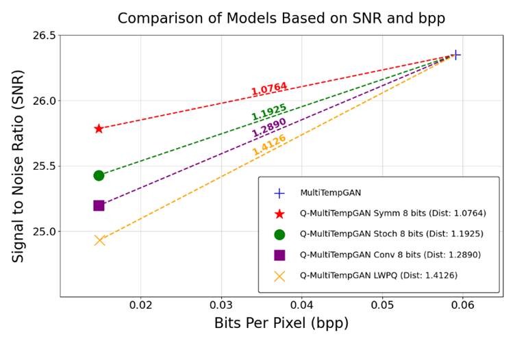
Figure 2: Comparison of different models based on their normalized SNR and bpp values.

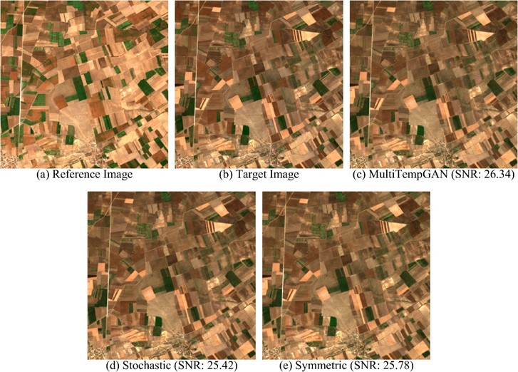
Figure 3: Visual comparison of reference, target, and reconstructed images using MultiTempGAN and Q-MultiTempGAN using Symmetric and Stochastic quantization with 8-bit precision.

The visual results in Figure 3 confirm the performance metrics discussed earlier, showcasing the outputs of the original MultiTempGAN model and its post-training quantized versions, including stochastic and symmetric quantization methods, alongside the reference and target images. The results demonstrate that the symmetric quantization method produces outputs closely aligning with the target image in terms of visual quality, highlighting its capability to achieve efficient image reconstruction without significant distortion.

6. Conclusion

Q-MultiTempGAN, despite the applied quantization strategies, continues to outperform other models such as LinkNet, ResNet, and U-Net, which were discussed in the original MultiTempGAN study. This shows the robust design of the MultiTempGAN framework and its ability to maintain high performance even under significant model compression.

SNR is a logarithmic metric measured in decibels (dB), meaning its values are not directly proportional to the underlying signal power. For instance, the average SNR of MultiTempGAN is 26.34, while that of the symmetric quantized version is 25.78. The perceived difference is not merely with the value of 0.56; rather, when calculated logarithmically, the difference in power corresponds to a percentage change, numerically reinforcing the closeness of the results.

Given the logarithmic nature of SNR, enhancing SNR while keeping bpp almost the same is critical for achieving better compression without sacrificing quality. Future research could explore advanced approaches like non-uniform quantization, which allows for more efficient allocation of bit-widths based on data (weights) distribution, potentially resulting in higher SNR with minimal memory overhead.

This study used TensorFlow 1.15 library, which lacks native support for Quantization-Aware Training (QAT) [21]. Future work could utilize newer versions of this library with QAT, where quantization is integrated during training. Unlike post-training quantization, QAT enables models to adapt to lower-precision weights while training, minimizing accuracy loss and achieving better trade-offs between accuracy and compression efficiency.

References

[1]. Huang, B. (Ed.). (2011). Satellite data compression. Springer New York.
[2]. Du, Q., & Fowler, J. E. (2007). Hyperspectral image compression using JPEG2000 and principal component analysis. IEEE Geoscience and Remote Sensing Letters, 4, 201-205.
[3]. Klimesh, M. (2005). Low complexity lossless compression of hyperspectral imagery via adaptive filtering. Interplanetary Network Progress Report, 42, 1-10.
[4]. Song, J., Zhang, Z., & Chen, X. (2013). Lossless compression of hyperspectral imagery via RLS filter. IET Electronics Letters, 49, 992-994.
[5]. The Consultative Committee for Space Data Systems (CCSDS). (2019). CCSDS123.0-B-2 recommended standard. Blue Book.
[6]. Liu, D., Li, Y., Lin, J., Li, H., & Wu, F. (2020). Deep learning-based video coding: A review and a case study. ACM Computing Surveys, 53, 1-35.
[7]. Dumas, T., Roumy, A., & Guillemot, C. (2018). Autoencoder-based image compression: Can the learning be quantization independent? In IEEE International Conference on Acoustics, Speech and Signal Processing (ICASSP) (pp. 1188-1192). IEEE.
[8]. Agustsson, E., Tschannen, M., Mentzer, F., Timofte, R., & Van Gool, L. (2019). Generative adversarial networks for extreme learned image compression. In IEEE International Conference on Computer Vision, Seoul, Korea.
[9]. Valsesia, D., & Magli, E. (2019). High-throughput onboard hyperspectral image compression with ground-based CNN reconstruction. IEEE Transactions on Geoscience and Remote Sensing, 57, 9544-9553.
[10]. Isola, P., Zhu, J. Y., Zhou, T., & Efros, A. A. (2017). Image-to-image translation with conditional adversarial networks. arXiv preprint arXiv:1611.07004.
[11]. Karaca, A. C., Kara, O., & Güllü, M. K. (2021). MultiTempGAN: Multitemporal multispectral image compression framework using generative adversarial networks. Journal of Visual Communication and Image Representation, 81, 103385. https://doi.org/10.1016/j.jvcir.2021.103385.
[12]. Copernicus. (n.d.). Sentinel-2 mission. Retrieved January 4, 2025, from https://sentiwiki.copernicus.eu/web/s2-mission.
[13]. European Space Agency (ESA). (n.d.). SNAP download. Retrieved January 4, 2025, from https://step.esa.int/main/download/snap-download.
[14]. Ronneberger, O., Fischer, P., & Brox, T. (2015). U-Net: Convolutional networks for biomedical image segmentation. In International Conference on Medical Image Computing and Computer-Assisted Intervention (pp. 234-241). Springer, Cham.
[15]. Chaurasia, A., & Culurciello, E. (2017). LinkNet: Exploiting encoder representations for efficient semantic segmentation. In 2017 IEEE Visual Communications and Image Processing (VCIP) (pp. 1-4). IEEE.
[16]. He, K., Zhang, X., Ren, S., & Sun, J. (2016). Deep residual learning for image recognition. In IEEE/CVF Conference on Computer Vision and Pattern Recognition (pp. 770-778).
[17]. Krishnamoorthi, R. (2018). Quantizing deep convolutional networks for efficient inference: A whitepaper. arXiv preprint arXiv:1806.08342.
[18]. Gholami, A., Kim, S., Dong, Z., Yao, Z., Mahoney, M. W., & Keutzer, K. (2021). A survey of quantization methods for efficient neural network inference. Proceedings of Machine Learning Research.
[19]. Jacob, B., Kligys, S., Chen, B., Zhu, M., Tang, J., Howard, A., ... Adam, H. (2018). Quantization and training of neural networks for efficient integer-arithmetic-only inference. In IEEE Conference on Computer Vision and Pattern Recognition (CVPR). https://doi.org/10.1109/CVPR.2018.00210.
[20]. Micikevicius, P., Narang, S., Alben, J., Diamos, G., Elsen, E., García, D., Phothilimthana, P., & LeGresley, P. (2018). Mixed precision training. In International Conference on Learning Representations (ICLR).
[21]. TensorFlow. (n.d.). Quantization-aware training. Retrieved January 4, 2025, from https://www.tensorflow.org/model_optimization/guide/quantization/training.
Cite this article
Gharagoz,N.S.;Karaca,A.C. (2025). Q-MultiTempGAN: Post-training Quantization of Multitemporal Multispectral Image Compression Models. Applied and Computational Engineering,100,154-162.
Data availability
The datasets used and/or analyzed during the current study will be available from the authors upon reasonable request.
Disclaimer/Publisher's Note
The statements, opinions and data contained in all publications are solely those of the individual author(s) and contributor(s) and not of EWA Publishing and/or the editor(s). EWA Publishing and/or the editor(s) disclaim responsibility for any injury to people or property resulting from any ideas, methods, instructions or products referred to in the content.
About volume
Volume title: Proceedings of the 5th International Conference on Signal Processing and Machine Learning
© 2024 by the author(s). Licensee EWA Publishing, Oxford, UK. This article is an open access article distributed under the terms and
conditions of the Creative Commons Attribution (CC BY) license. Authors who
publish this series agree to the following terms:
1. Authors retain copyright and grant the series right of first publication with the work simultaneously licensed under a Creative Commons
Attribution License that allows others to share the work with an acknowledgment of the work's authorship and initial publication in this
series.
2. Authors are able to enter into separate, additional contractual arrangements for the non-exclusive distribution of the series's published
version of the work (e.g., post it to an institutional repository or publish it in a book), with an acknowledgment of its initial
publication in this series.
3. Authors are permitted and encouraged to post their work online (e.g., in institutional repositories or on their website) prior to and
during the submission process, as it can lead to productive exchanges, as well as earlier and greater citation of published work (See
Open access policy for details).