


1. Introduction
In recent years, unsupervised learning models have been obtained increasingly attention in the field of deep learning, especially in deep generative models, which have made great progress.
Variational auto-encoder is a deeply latent space generation model, which has revealed tremendous application in data generation, particularly in graphic generation. However, traditional VAE uses the approximate a Nacherleben posteriori distribution of the latent variables instead of the a priori distribution in the coding process, which greatly limits the learning ability of the hidden variables, and the generated images are blurred and less expressive for complex models. VAEs combined with GAN can synthesize high-quality images, almost overcoming the shortcomings of traditional VAEs in generating blurred images. Since then, more and more researches have been conducted to make the influencing factors of the nature of the VAE mechanism clearer and better structured,
2. Background
2.1. Autoencoders
The Auto-Encoders [1], regard as a self-supervised learning model, is primarily used in data dimensionality reduction, image noise reduction, and image sort . The input and output expectations of the auto-encoders are unlabeled samples, while the output of the implicit layer is an abstract feature representation of the samples. The autoencoder first accepts the input sample, converts it into an efficient abstract representation, and then outputs a reconstruction of the original sample.
The encoder maps the high level input samples to the status abstract representation to achieve compression and dimensionality reduction of the samples, while the decoder converts the abstract representation to the desired output to achieve reconstruction of the original input samples. Its structure is shown in Figure 1.
|
Figure 1. AE shecmatic diagram. |
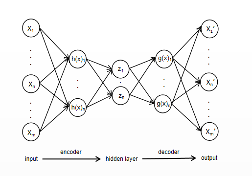
The orig. input X is encoded by the encoder h to form the set X', i.e., X' = h(X); the decoder f decodes X' to generate the orig. data X, After repeated training, the self-encoder tries to copy the input to the output. However, the self-encoder should not be designed so that the inputs are exactly equal to the outputs, otherwise, the self-encoder would be useless. To put it another way, the output data it supposed to approximately equivalent to the input, which demands imposing restraints on the self-encoder. Giving rise to the self-encoder tends to learn valid features of the data and discard irrelevant features.
After training, the self-encoder will gradually output samples that approximate the original input, but it should not be trained too thoroughly, otherwise, the self-encoder will only produce results that are almost identical to the input samples. Such an approach can lead to severe overfitting Hence, it is imperative to add some constraints to the auto-encoder to ensure that the output is not exactly equivalent to the input. These restrains compel the self-encoder to think about which parts of the input demand to replicated and which parts require to be weighted down or discarded, consequently, the self-encoder tends to learn the effective features and discard the uncorrelated features.
2.2. Variational Auto-Encoders
|
Figure 2. CVAE shecmatic diagram. |

Variational self-encoder is a generative network structure on account of variational Bayesian inference which put forward by Kingma et al [2] in 2014. VAE looks resemble to AE, however, the principle is completely different. VAE uses two neural networks, encoder and decoder, to build two probability density distribution models: encoder used for variational ratiocination of the foregone input data to produce a variational probability distribution of the latent variable, named the inference network; the other reduces the produced probability distribution on account of the produced Gaussian variational probability distribution of the hidden variable to generate an approximative approximate probability distribution with the primitive data, called the generation network. The model is shown in the figure2.
In Figure 2, Z is the hidden variable, qϕ(z|x) and Pθ(z)Pθ(x'|z) are the conditional distributions learned by the encoding and decoding processes, which are the recognition pattern and the generation pattern.
In the recognition model, since the distribution of the hidden variable Z is not directly observable and cannot be solved by variational inference using the EM algorithm directly, to solve this problem, VAE introduces an identification pattern qϕ(z|x) in the inferential network to replace the true posterior distribution Pθ(z|x) which cannot be computed precisely, and supports that the identification model qϕ(z|x) is a foregone modality of distribution such that qϕ(z|x) can be The training objective of VAE is to minimize the distance between the input sample distribution p(X) and the confiscated sample distribution p(X’)in order to make the two approximately equal, VAE uses KL scatter to express the pixel low between the two and minimizes it by majorizating the restraint arguments θ and Φ.
DKL(P(X)|P(X’)) = P(X) \( \frac{P(X)}{P(X \prime )} \) dx (1)
However, due to the unknown nature of the true distribution, the KL scatter cannot be calculated directly, so VAE introduces the approximate posterior distribution qϕ(z|x) , and uses the maximum likelihood method is used to optimize the objective function and derive its log-likelihood function
logP(X) =DKL(qϕ(z|x)||Pθ(z|x))+L(ϕ,θ;X) (2)
Since the KL dispersion is constantly greater than 0, L(ϕ,θ;X) becomes the variational lower bound of the likelihood function
L(ϕ,θ;X) == Eqϕ(z|x)[-log qϕ(z|x) + log Pθ(x, z)) (3)
From equation(2) and equation(3),we can derive its loss function as :
JVAE =DKL(qϕ(z|x)||Pθ(z|x)) - Eqϕ(z|x)(lb(Pθ(X|Z))) (4)
After introducing the identification model qϕ(z|x) instead of Pθ(z|x), the latent variable Z is assumed to be stochastically sampled from the foregone distribution qϕ(z|x), and introduced an ancillary arguments ε to convert the distribution of qϕ(z|x) to derive gϕ(ε, x) thus make z = gϕ(ε, x), where
ε ~p(ε) and p(ε) has a foregone minor likelihood distribution. Assume that qϕ(z|x) follows the ordinary normal distribution hence , Z’s sampling can be accomplished by
zi = μi + σi ∙ εi (5)
Making Pϕ(z) ~ N(0,1) , and only one sample of data is sampled at a time, so the variational lower bound L(ϕ,θ;X) can be simplified as
L(ϕ,θ;X) = ∑[lb(σi)2-(μi)2-(σi)2+1]+lbPθ(xi’|zi) (6)
The introduction of ancillary arguments makes the relation between the latent variate z and σ, μ from sampling compute to numerical compute, which can be directly optimized using random gradient descent. The conditional distribution Pθ(xi'|zi) obeys the Bernoulli distribution or Gaussian distribution, and its mean and standard deviation can be calculated by the neural network, then Pθ(xi'|zi) is enable to computed on the basis of its probability density function formula. At this point, each of the variational floor limit is enable to computed directly.
3. Variant forms of variational auto-encoders
Variational auto-encoders is considered as a hybrid of neural networks and Bayesian networks, and have many advantages over traditional deep generative networks.
However, VAE still has many shortcomings. On the one hand, the generated images are often blurred and poorly represented for complex models. At the same time, the encoding process of using the approximate posterior distribution Pθ(z|x) of the hidden variables instead of the prior distribution Pθ(z) greatly limits the learning of the hidden variables.
In recent years, more and more VAE variants have been proposed to correspond to the shortcomings of traditional VAE as well as to the increasingly complex requirements.
Table 1. The typical VAE variants in recent years.
serial number | name | abbreviate | Year of presentation |
1 | Variational Autoencoders | VAE | 2014 |
2 | Conditional Variational Autoencoders | CVAE | 2015 |
3 | Variational Fair Autoencoder | VFAE | 2015 |
4 | Importance-Weighted Autoencoders | IWAE | 2015 |
5 | Variational Autoencoders with GAN | VAE-GAN | 2016 |
6 | Conditional Variational Autoencoders with GAN | CAE-GAN | 2017 |
7 | Variational Lossy Autoencoders | VLAE | 2017 |
8 | Channel-Recurrent Variational Autoencoders | CRVAE | 2017 |
9 | Least Square Variational Bayesian Autoencoders | LSVAE | 2017 |
10 | Information Maximizing Variational Autoencoder | IMVAE | 2017 |
11 | Multi-Stage Variational Auto-Encoders | MSVAE | 2017 |
12 | Wake-Sleep Variational Autoencoders | WSVAE | 2017 |
13 | Nonparametric Variational Autoencoders | NpVAE | 2017 |
14 | Memory-enhanced Variational Autoencoders | MeVAE | 2017 |
15 | Fisher Autoencoders | FAE | 2018 |
16 | Autoencoder with support vector data description | VAE-SVDD | 2020 |
3.1. Conditional Variational Autoencoders
VAE maps the samples into probability distributions. That is, the mean and variance of the output distribution are output and the decoder decodes the latent variable z sampled from that division. Due to the introduction of variance, the sampled latent variables have some uncertainty, and although it is possible to generate similar outputs from the input samples, it does not control their directional generation into a specific class of sample data. In 2014, makhzani et al. proposed Conditional Variational Autoencoder [3], which differs from the VAE in that the input data of CVAE adds category information Y for controlling the generation of category-specific samples, in addition to the original data samples X.
|
Figure 3. CVAE shecmatic diagram. |
From Figure 3, it is easy to see that the structure of CVAE is similar to that of VAE with only the addition of the input data category information Y. CVAE also changes from the unsupervised mode of VAE to the semi-supervised mode.
Similarly, the loss function of CVAE is not much different from that of VAE, both of which maximize the log marginal likelihood by maximizing the variational floor limit.
LCVAE(x,y;ϕ,Θ)=-DKL(qϕ(z|x)||Pθ(z|x))+ \( \frac{1}{L}\sum _{l=1}^{L}p \) θ(y|x,zl) (6)
due to the introduction of the category control unit, the CVAE can control the production of directional image data.By changing the category information of the encoder network input, CVAE can control the transformation of the digital image from a certain number to a specific number.
However, CVAE with the addition of category information control achieves the goal of being able to synthesize image data directionally it still does not solve the shortcomings of VAE itself: blurred generated images, low accuracy of synthesized image data, and poor performance when encountering complex data models.
3.2. Variational Fair Autoencoder
VFAE is another semi-supervised model with labels after CVAE, it was proposed by Louizos et al. in 2015[4], and its purpose is to separate the noise in the data samples from the information of the hidden variables, so that the model learns more explicitly the feature representation of certain non-variable factors, and VFAE hopes to improve the accuracy of the hidden variable Z by separating the noise S as much as possible in the learning process of the hidden variable Z.FAE was proposed by Louizos et al. in 2015, aiming in separate the noise from the hidden variable information in the data sample, allowing the model to learn more explicitly the characteristic representation of certain non-variable factors.
Intersecting with the traditional VAE, VFAE proposes to add Maximum Mean Discrepancy as the regular term and derive the penalty term from the posterior distribution qϕ(z|s) of the hidden variable Z obtained from the noise S, and let qϕ(z|s) as small as possible, which can effectively reduce the dependence between the noise S and the hidden variable Z.
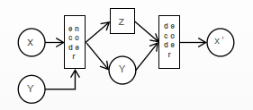
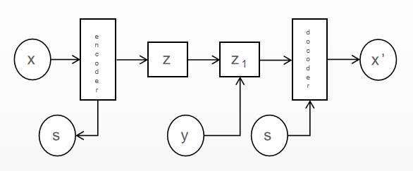
However, the noise itself may have some association with the category information, and only separating the noise without doing any operation on the category information may have some effect on the overall model effect. Therefore, VFAE adds a new hidden variable layer Z1 after the original hidden variable layer Z. The sample data are encoded to get the hidden variable that separates the noise, and then the category information Y is re-added to Z to get Z1, thus reducing the affected degree of category information.
|
Figure 4. VFAE shecmatic diagram. |
3.3. Variational Autoencoders with GAN
Although there have been many variants with various improvements to the traditional VAE, they still do not solve the problem of blurred VAE-generated images. Meanwhile, VAE started to be used for anomaly detection, but VAE focuses more on generating similar samples rather than detecting anomalous samples.
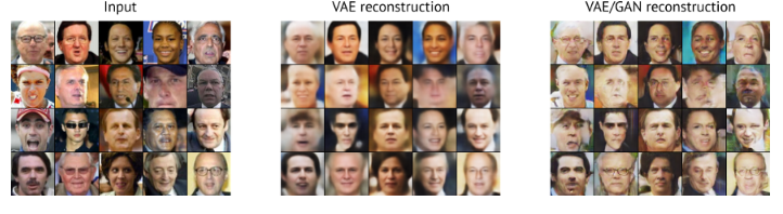
Anders et al. proposed a self-adversarial mechanism by combining adversarial generative networks GANs [5], which effectively ensures the quality of the generated image.
|
Figure 5. Original image and reconstructed image by VAE, VAE-GANs. |
Just like VAE, GANs also belong to generative algorithms under unsupervised machine learning. A classical GAN network consists of a generative neural network and a discriminative neural network. The former receives noise as input and generates samples, while the discriminative neural network evaluates and discriminates these samples generated from the training samples. Much like the VAEs, the generating networks also use latent variables and arguments to describe the data distribution.
The main goal of the generator is to deceive the recognition neural network - to reduce the discrimination correctness of the recognition neural network. This can be achieved by continuously generating samples from the training data distribution. This is very similar to the real-life tug-of-war between police and cybercriminals. The cybercriminals (generators) create many fake identities to masquerade as ordinary citizens, while the police (recognizers) need to discriminate between real and fake identities.
|
Figure 6. VAE-GAN shecmatic diagram. |
3.4. Conditional Variational Autoencoders with GAN
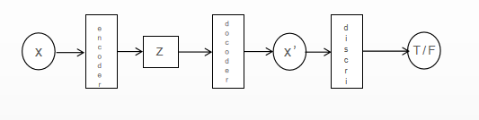
In 2017, BAO [6] et al. added the discriminator [7] in the GAN model after the decoder to ensure that the images generated by CVAE have high quality.
|
Figure 7. CVAE-GAN shecmatic diagram. |
|
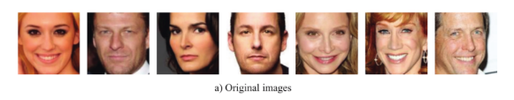
Figure 8. original images.
|
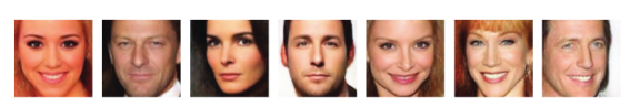
Figure 9. CVAE-GAN reconstructed images. |
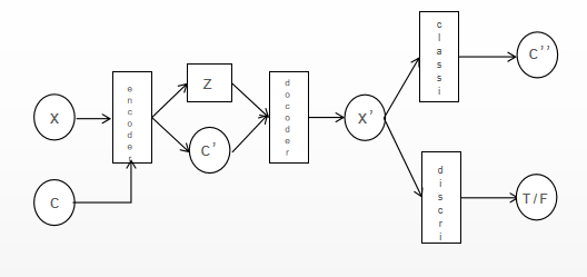
The loss function of CVAE-GAN is:
LCVAE-GAN =λ1LKL+λ2LG+λ3LGD+λ4LGC +LD+LC (7)
λ i are four hyperparameters which are set to λ1 =1,λ2 = 1, λ3 = 10-3 , λ4 = 10-3.
LKL is the loss function of the original CVAE, which represents the KL scatter of the identification model qϕ(z|x,c) with the prior distribution of the hidden variable Z.
LG denotes the sum of reconstruction loss and feature matching loss of the decoder generated sample X' and the real sample X.
LGC represents the sum of reconstruction loss and feature matching loss of the decoder generated sample X' and the real sample X.
LD represents the game loss of discriminator and generative network GANs.
LC denotes the category classification loss of the networkclassifier.
CVAE-GAN has shown good generation results in image synthesis experiments and can obtain high quality synthetic images.
3.5. Fisher Autoencoders
In contrast to other VAE variants that seek to improve network structure or noise separation, FAE’s direction is more specific in that it attempts to clearly explain the workings of VAE from an information-theoretic perspective, and FAE[8] shows that any encoding-decoding-based model of hidden variable space generation inherently receives control of the “Fisher-Shannon information trade-off”
By adjusting the Fisher-Shannon information, the relationship between marginal likelihood estimates and data-hidden variable dependence can be balanced and improve the expression of the model.
The breakthrough of FAE compared with VAE is to propose the importance and interrelationship of Fisher information quantity and Shannon information entropy played in VAE:
N(X)∙ J(X) ≥ K , K is a constant and K >1 (8)
Fisher information quantity J(X) influences the parameter estimation, and Shannon information entropy N(X) influences the dependence between data and Z in the training process for the hidden variable Z.
The variational lower bound of FAE adds an equation to VAE:
Lin = λz|J(z) - Fz| - λx'|J(x') - Fx'| (8)
J(X’) denotes the Fisher information quantity; Fz denotes the precision of the Fisher information quantity control parameter estimation, the larger Fz denotes the more precise parameter estimation, the larger the Fisher information quantity, the corresponding entropy power will be reduced.
There is no doubt that FAE offers a new and improved direction for VAE.
3.6. Other variants of VAEs
Since the Variational Self-Encoder is effective in automatically extracting features, improving the complexity of traditional methods of extracting features and avoiding overfitting, VAE has been used in more and more aspects in recent years, and there are far more VAE variants applied to different aspects in different fields.
In addition to the VAE variants described above, there are also multi-stage variational self-encoders MSVAE [9] for fine-grained image generation, least squares discriminative self-encoders LSVAE [10] using least squares loss as a regular penalty term, and adVAE [11] by adding a self-adversarial mechanism, VAEs and variants are playing an increasing role.
In addition to image generation, VAE is also applicable to anomaly detection, from traditional VAE, to VAE-GAN, to VAE-svdd proposed in 2021, which incorporates the deep-svdd judgment mechanism. In music, WSVAE [12], a wake-to-sleep variational self-encoder applicable to the generation of sequential language data, etc., are based on different needs of practical applications. The proposed improved models.
4. Conclusion
Since its introduction in 2014, VAE and its variants have been increasingly used especially in data generation. As the data continues to grow huge, traditional VAE can no longer meet the needs of people and more and more VAE variants have started to be proposed. The improvement of VAE mainly focuses on three aspect, first, amend the loss function: the KL scattering regular penalty term used in traditional VAE give rise to the model in the hidden space boundary expression vague and the penalty effect is not obvious, which makes the generated image inaccurate . Subsequently, whether LSVAE, NVAE, or FAE using Fisher-Shannon information entropy, better loss functions are proposed to make the hidden space boundary clearer, thus effectively improving the disadvantage of blurred generated images. Second, optimized network structure: Another problem of VAE is that the model first fits the data to a Gaussian distribution, and when we select P, KL is already theoretically impossible to approach 0 infinitely, so we can only get an average but mediocre result in the end. Therefore either by combining VAE-GAN of GAN, adVAE which introduces a self-adversarial mechanism, or VAE-svdd which adds X is a deepening of the traditional VAE network structure and implicitly abandons the assumption that Q is Gaussian distributed and replaces it with a more general distribution, thus improving the generation effect. Third, information separation: Information separation aims to purify the noise information in the hidden variable space, and both hope to weaken the dependence between information and make less interference between each other, thus improving the expression effect of VAEs. The purpose of this paper is to facilitate a general understanding and grasp of VAE models and their development, and we hope this will be helpful for them.
References
[1]. BOURLARD H, KAMP Y. Auto-association by multilayer perceptrons and singular value decomposition[J] Biological Cybernetics, 1988, 59(4/5): 291-294.
[2]. Kingma D Welling. Auto-encoding variational bayes[C]// International Conference on Learning Repre- sentations, 2014.
[3]. Makhzani A, Shlens J, Jaitly N, et al. Adversarial autoen- coders[J]. arXiv:1511.05644, 2015.
[4]. Louizos C, Swersky K, Li Y et al. The variational fair autoencoder[J]. arxiv: 1511.00830, 2015.
[5]. Anders Boesen Lindbo Larsen, Søren Kaae Sønderby, Hugo Larochelle, Ole Winther Autoencoding beyond pixels using a learned similarity metric[C]. arXiv: 1512.09300.2016.
[6]. Jianmin Bao, Dong Chen, Fang Wen, Houqiang Li, Gang Hua, CVAE-GAN: Fine-Grained Image Generation through Asymmetric Training[J]. arXiv :1703.10155.2017.
[7]. Mescheder L, Nowozin S, Geiger A.Adversarial varia- tional Bayes: unifying variational autoencoders and gen- erative adversarial networks[J]. arXiv: 1701.04722.2017.
[8]. Zheng Huangjie, Jiangchao Yao, Zhang Ya,et al. Under-standing VAEs in Fisher_Shanon plane[J]. arXiv: 1807.03723.2018.
[9]. Cai Lei, Gao Hongyang, Ji Shuiwang. Multi-stage varia-tional auto-encoders for coarse-to-fine image generation[J]. arXiv: 1705.07202,2017.
[10]. Ramachandra G. Least square variational Bayesian auto- encoder with regularization[J]. arXiv: 1707.03134, 2017.
[11]. Xuhong Wang, Ying Du, Shijie Lin, Ping Cui, Yuntian Shen, adVAE: A self-adversarial variational autoencoder with Gaussian anomaly prior knowledge for anomaly detection.
[12]. Shen Xiaoyu, Su Hui, Niu Shuzi, et al. Wake-sleep varia- tional autoencoders for language modeling[C]//International Conference on Neural Information Processing, 2017, 405-414.
Cite this article
Liu,J. (2023). Review of variational autoencoders model. Applied and Computational Engineering,4,588-596.
Data availability
The datasets used and/or analyzed during the current study will be available from the authors upon reasonable request.
Disclaimer/Publisher's Note
The statements, opinions and data contained in all publications are solely those of the individual author(s) and contributor(s) and not of EWA Publishing and/or the editor(s). EWA Publishing and/or the editor(s) disclaim responsibility for any injury to people or property resulting from any ideas, methods, instructions or products referred to in the content.
About volume
Volume title: Proceedings of the 3rd International Conference on Signal Processing and Machine Learning
© 2024 by the author(s). Licensee EWA Publishing, Oxford, UK. This article is an open access article distributed under the terms and
conditions of the Creative Commons Attribution (CC BY) license. Authors who
publish this series agree to the following terms:
1. Authors retain copyright and grant the series right of first publication with the work simultaneously licensed under a Creative Commons
Attribution License that allows others to share the work with an acknowledgment of the work's authorship and initial publication in this
series.
2. Authors are able to enter into separate, additional contractual arrangements for the non-exclusive distribution of the series's published
version of the work (e.g., post it to an institutional repository or publish it in a book), with an acknowledgment of its initial
publication in this series.
3. Authors are permitted and encouraged to post their work online (e.g., in institutional repositories or on their website) prior to and
during the submission process, as it can lead to productive exchanges, as well as earlier and greater citation of published work (See
Open access policy for details).
References
[1]. BOURLARD H, KAMP Y. Auto-association by multilayer perceptrons and singular value decomposition[J] Biological Cybernetics, 1988, 59(4/5): 291-294.
[2]. Kingma D Welling. Auto-encoding variational bayes[C]// International Conference on Learning Repre- sentations, 2014.
[3]. Makhzani A, Shlens J, Jaitly N, et al. Adversarial autoen- coders[J]. arXiv:1511.05644, 2015.
[4]. Louizos C, Swersky K, Li Y et al. The variational fair autoencoder[J]. arxiv: 1511.00830, 2015.
[5]. Anders Boesen Lindbo Larsen, Søren Kaae Sønderby, Hugo Larochelle, Ole Winther Autoencoding beyond pixels using a learned similarity metric[C]. arXiv: 1512.09300.2016.
[6]. Jianmin Bao, Dong Chen, Fang Wen, Houqiang Li, Gang Hua, CVAE-GAN: Fine-Grained Image Generation through Asymmetric Training[J]. arXiv :1703.10155.2017.
[7]. Mescheder L, Nowozin S, Geiger A.Adversarial varia- tional Bayes: unifying variational autoencoders and gen- erative adversarial networks[J]. arXiv: 1701.04722.2017.
[8]. Zheng Huangjie, Jiangchao Yao, Zhang Ya,et al. Under-standing VAEs in Fisher_Shanon plane[J]. arXiv: 1807.03723.2018.
[9]. Cai Lei, Gao Hongyang, Ji Shuiwang. Multi-stage varia-tional auto-encoders for coarse-to-fine image generation[J]. arXiv: 1705.07202,2017.
[10]. Ramachandra G. Least square variational Bayesian auto- encoder with regularization[J]. arXiv: 1707.03134, 2017.
[11]. Xuhong Wang, Ying Du, Shijie Lin, Ping Cui, Yuntian Shen, adVAE: A self-adversarial variational autoencoder with Gaussian anomaly prior knowledge for anomaly detection.
[12]. Shen Xiaoyu, Su Hui, Niu Shuzi, et al. Wake-sleep varia- tional autoencoders for language modeling[C]//International Conference on Neural Information Processing, 2017, 405-414.