1. Introduction

Time series modeling is critical across numerous domains, including healthcare, energy, and finance [1-2], where capturing temporal dependencies and multi-scale patterns is essential for accurate forecasting. Predicting future trends and patterns enables informed decision-making, efficient resource allocation, and effective risk management, making time series forecasting an indispensable tool in industry.

Financial time series forecasting, particularly for stock market data, presents significant challenges due to the unique characteristics of such data. Stock series are influenced by many factors, including market sentiment, geopolitical events, and economic indicators [3], resulting in high levels of noise and making it difficult to distinguish meaningful signals from random fluctuations. Additionally, financial time series are often non-stationary, exhibit volatility clustering, and contain nonlinear patterns. These characteristics all complicate the model.

Statistical and machine learning (ML) models have been widely used for stock time series forecasting. However, statistical models may lose effectiveness when their strong assumptions are violated, while ML models may struggle to capture the intricate patterns necessary for real-world trading scenarios. Deep learning (DL) approaches have gained prominence due to their ability to extract features from complex data and their reliance on fewer assumptions. Despite these advancements, DL models still face the problem of high dimensionality, particularly when dealing with a stock market that incorporates numerous variables to capture dynamic market behaviors. Furthermore, most DL models are limited to single-task learning, restricting their ability to leverage shared information across related tasks.

To address these limitations, this paper proposed a multi-task learning (MTL) model for stock time series forecasting, which simultaneously predicts trading volume, closing price, and volatility. By leveraging shared information across related tasks, the MTL model provides a more comprehensive approach to modeling stock market behavior. The proposed model incorporates CNN, LSTM, and the attention mechanism as shared layers to extract correlated features, while task-specific layers capture individual task characteristics. This MTL model, built on a deep learning framework, is evaluated against benchmark models to demonstrate its performance and generalization ability.

2. Literature Review

There are three key methods widely applied in financial time series forecasting, which are the classical statistical method, single-task machine learning method, and multi-task learning method.

2.1. Statistical Method

Statistical models have been widely used for stock price forecasting. Mondal et al. proposed an ARIMA model for stock price prediction across 56 datasets from various sectors, achieving over 85% accuracy and demonstrating strong generalization and interpretability [4]. However, ARIMA models face limitations, such as their inability to capture fat-tailed distributions, handle volatility clustering, and adapt to non-stationary data [5]. To address these issues, Vasudevan and Vetrivel built GARCH-type models, showing that the EGARCH model outperforms symmetric GARCH in forecasting the conditional variance of stock returns [6].

2.2. Single-task Machine Learning Method

Recent developments in deep learning have greatly enhanced stock market prediction by capturing nonlinear patterns and extracting features from noisy data. A comparative study of ARIMA, LSTM, and BiLSTM models, applied to six stock datasets, revealed that deep learning models reduced RMSE by more than 80% compared to ARIMA [7]. To more effectively capture both linear and nonlinear patterns, researchers have developed a hybrid model, ARIMA-ANN, which requires no strong assumptions and outperforms individual models as well as earlier hybrid approaches, particularly on highly fluctuating datasets [8]. Mei et al. further advanced this approach by proposing an ARIMA-SVM model, where ARIMA prediction errors serve as inputs to SVM, achieving over 90% accuracy on IBM stock data [9].

2.3. Multi-task Learning Method

Multi-task learning (MTL) enhances model performance by leveraging shared information across related tasks. In computer vision, Ranjan et al. developed an MTL model for simultaneous face detection, landmark localization, pose estimation, and gender recognition [10]. Similarly, Samala et al. applied MTL for breast cancer detection, achieving high AUC score [11]. In finance, Ma and Tan proposed an MTL framework for forecasting multiple related stocks simultaneously, outperforming baseline methods [12]. Yuan et al. designed an MTL model for stock market forecasting during COVID-19, effectively capturing internal and external market features [13]. These studies highlight the benefits of MTL in extracting shared patterns and improving generalization.

3. Methodology

3.1. Data Source

The dataset, sourced from Alpha Vantage API, spans from 2010 to the most recent data. The 2008 financial crisis period is excluded due to its minimal impact on current data, while the COVID-19 period is included in the ongoing economic effects.

3.2. Autoregressive Integrated Moving Average (ARIMA)

ARIMA model is a widely used statistical method for univariate time series forecasting, combining three components: Autoregressive (AR), Integrated (I), and Moving Average (MA). The model is denoted as ARIMA(p, d, q), where p is the order of the AR component, d is the degree of differencing, and q is the order of the MA component.

The AR(p) component models the relationship between the current value ( \( {Y_{t}} \) ) and its past values:

\( {Y_{t}}=c+ {{φ_{1}}Y_{t-1}}+{{φ_{2}}Y_{t-2}} +…+ {{φ_{p}}Y_{t-p}}+ {ε_{t}} \) (1)

where \( c \) is a constant, \( {φ_{1}}, {φ_{2}}, {…, φ_{p}} \) are autoregressive parameters, and \( {ε_{t}} \) is the error term at time \( t \) .

The MA(q) component models the relationship between the current value ( \( {Y_{t}} \) ) and past error terms:

\( {Y_{t}}=μ + {{θ_{1}}Y_{t-1}}+{{θ_{2}}Y_{t-2}} +…+ {{θ_{q}}Y_{t-q}}+ {ε_{t}} \) (2)

where \( μ \) is the mean of series, \( {θ_{1}}, {θ_{2}}, {…, θ_{p}} \) are moving average parameters, and \( {ε_{t}} \) is the noise term.

Differencing (degree d) removes trends and seasonality to make the series stationary, where the degree represents the number of times differencing is taken [14]. \( \)

AR component captures the memory of the time series, detecting strong temporal dependencies [14], while the MA component captures the shocks, detecting the sudden changes or irregularities [15]. As a result, AR and MA are combined to effectively address more complex time series. When the series is stationary, the ARIMA model can be expressed as,

\( {Y_{t}}= c+ {{φ_{1}}Y_{t-1}}+{{φ_{2}}Y_{t-2}} +…+ {{φ_{p}}Y_{t-p}}+ {{θ_{1}}Y_{t-1}}+{{θ_{2}}Y_{t-2}} +…+ {{θ_{q}}Y_{t-q}}+ {ε_{t}} \) (3)

In this study, three ARIMA models are developed. The optimal parameter d is determined using the Augmented Dickey-Fuller test, while p and q are selected via grid search guided by Autocorrelation Function (ACF) and Partial Autocorrelation Function (PACF) plots.

3.3. Deep Learning Neural Networks

Convolution Neural Networks (CNN) can be used to perform feature extractions, learning through filter optimization [16]. In this study, three types of layers are used: Convolutional layer applies learnable filters to extract local patterns, pooling layer reduces dimensionality while preserving key features, and flatten layer converts feature maps into a 1D vector for fully connected layers.

Recurrent Neural Network (RNN) is commonly used to process sequential data by maintaining a hidden state that captures information from the previous time steps [17]. The standard neural networks have limited memory about previous data and only utilize the current input to forecast. But the neurons in RNN can recur a hidden variable \( {h_{t}} \) , containing information that later iterations can use. The update process can be expressed mathematically as follows,

\( {h_{t}}=f({W_{h}} ∙ {h_{t-1}}+ {W_{x}} ∙ {x_{t}}+ {b_{h}}) \) (4)

\( {y_{t}}=f({W_{y}} ∙ {h_{t}}+ {b_{y}}) \) (5)

where \( {W_{h}}, {W_{x}}, {W_{y}} \) are weights, \( {b_{h}}, {b_{y}} \) are bias terms, \( {x_{t}}, {y_{t}} \) are input and output at time step \( t \) , and \( f \) is activation function.

Long Short-Term Memory (LSTM) is a type of RNN that can address the vanishing gradient problem of traditional RNNs, using memory cells and gating mechanisms (forget gate, input and output gate) to capture long-term dependency, learning when to remember the information that is needed in later processing and when to forget the information that is no longer required [18].

Attention is a mechanism that determines the relative importance of each element in the sequence. It can resolve the weakness of RNN in leveraging the information of hidden layers, where it places higher importance on information from recent layers, compared with those from earlier layers.

In this paper, the univariate deep learning models are LSTM-based, incorporating dropout, batch normalization, and L2 weight regularization to prevent overfitting. They are trained with Adam optimizer and optimized via MSE loss.

3.4. Multi-task Learning (MTL)

MTL model can improve task performance by leveraging shared information across tasks. Given M related or at least partially related learning tasks, \( \lbrace {T_{i}}\rbrace _{i=1}^{M} \) , MTL is trying to enhance the training of \( {T_{i}} \) from learning some or all M tasks. The MTL loss is a weighted combination of individual task losses \( {L_{i}} \) , the simultaneous optimization of loss function across all tasks can lead to a significant improvement in model performance [19].

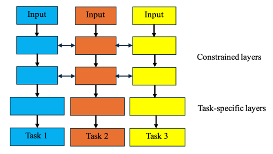
In the deep learning context, the MTL structure is categorized into two types, hard and soft parameter sharing. For hard parameter sharing in Figure 1, the shared layers can extract common features that are beneficial for all tasks, while task-specific layers receive common features as inputs and learn unique features. It can reduce overfitting by promoting generalized representations. For soft parameter sharing in Figure 2, each task maintains its own parameters, while a feature-sharing mechanism facilitates the information sharing between tasks [20].

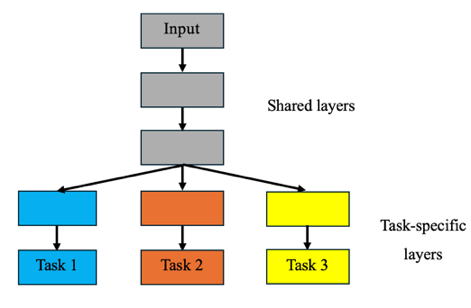
This paper employs a hard parameter sharing structure. The shared layers comprise a CNN block for localized temporal dependencies and an LSTM network with an attention mechanism for enhanced sequence representation. The extracted features are subsequently directed into task-specific branches: a dense network with residual connections for closing price prediction and LSTM branches for forecasting trading volume and volatility. To mitigate overfitting, the model integrates Dropout and Batch Normalization layers. Hyperparameter tuning and loss weight optimization are utilized to further enhance predictive performance across tasks.

3.5. Data Preprocessing and Model Training

The dataset includes five variables: closing price, opening price, low price, high price, and volume. Closing price and volume are used as the target variables. The volatility variable is computed as the rolling standard deviation of log returns, where log returns is calculated as:

\( Log Returns= log{(\frac{{Closing Price_{t}}}{C{Closing Price_{t-1}}})} \) (6)

A 20-day rolling window is applied, and the standard deviation is annualized by multiplying by \( \sqrt[]{252} \) (assuming 252 trading days per year).

To enhance model performance, technical indicators are added, providing additional information about market trends, which can be leveraged by the multi-task learning model. These indicators were selected based on their established relevance in financial time series analysis and their ability to capture different aspects of market behavior. Moving average (MA) and relative strength index (RSI) are added, where MA can capture long-term trends by smoothing price fluctuations and RSI can identify overbought or oversold, signaling potential price reversals. On-balance volume (OBV) can indicate market sentiment and anticipate potential volume spikes or drops, and Average True Range (ATR) can measure the price volatility, reflecting market uncertainty.

For data preprocessing, the data is normalized using MinMaxScaler and converted to sequence format for deep learning model inputs. The dataset is split into training, validation, and test sets in an 8:1:1 ratio, preserving the chronological order of the time series.

Three ARIMA models and three single-task deep learning models (DL) are developed as benchmarks for performance comparison. Each DL model is trained on the training set, with hyperparameters tuned on the validation set using grid search. Predictions are made on the test set and transformed back to their original scales due to prior normalization. For the MTL model, hyperparameters are optimized using a random search through the Keras Tuner library. This algorithm was used to explore different hyperparameter combinations to minimize the validation loss.

4. Results

Evaluation metrics are carefully chosen to align with the characteristics of the forecasting tasks. MAE and RMSE are employed, as MAE provides an intuitive measure of average error magnitude, while RMSE emphasizes large deviations, penalizing extreme errors. MAPE is also utilized as a criteria, as it offers a normalized error measure, particularly useful for trading volume data with spikes and anomalies.

The experimental results, comparing the MTL model with benchmarks (ARIMA and DL), are presented in Table 1 (trading volume), Table 2 (closing price), and Table 3 (volatility). Visual comparisons of the results are shown in Figure 3 (trading volume), Figure 4 (closing price), and Figure 5 (volatility).

Table 1: Trading volume forecasting results.

Table 2: Closing price forecasting results. Table 3: Volatility forecasting results.

The MTL model outperforms both DL and ARIMA across all tasks. For volume forecasting, the MTL model achieves the lowest MAE (8678394.180), representing a 9.2% error relative to the mean trading volume (94719750), compared to DL (10.1%) and ARIMA (31.6%). It also achieves the lowest MAPE and RMSE, demonstrating superior accuracy and robustness. For closing price forecasting, the MTL model achieves the lowest MAE (0.933), representing a 3.9% error relative to the mean price 23.728, compared to DL (4.3%) and ARIMA (35.6%). Similarly, it achieves the lowest MAPE and RMSE. In volatility forecasting, the MTL model achieves the lowest MAE (0.018), representing a 6.0% error relative to the mean volatility (0.302), along with the lowest MAPE (0.077) and RMSE (0.027).

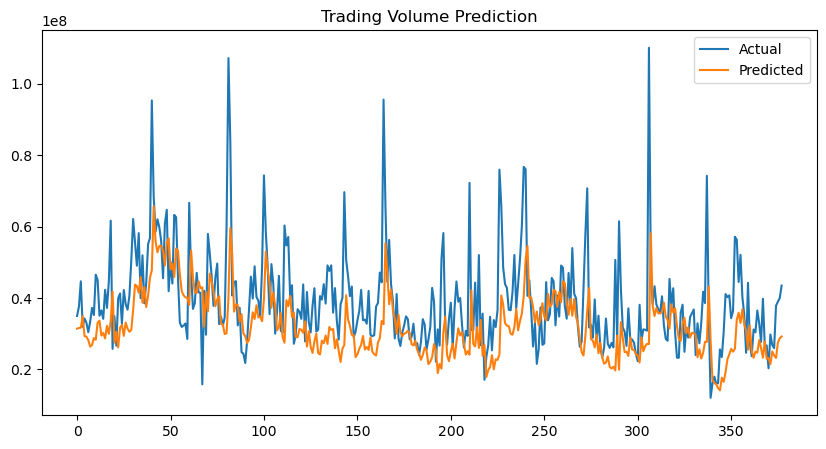
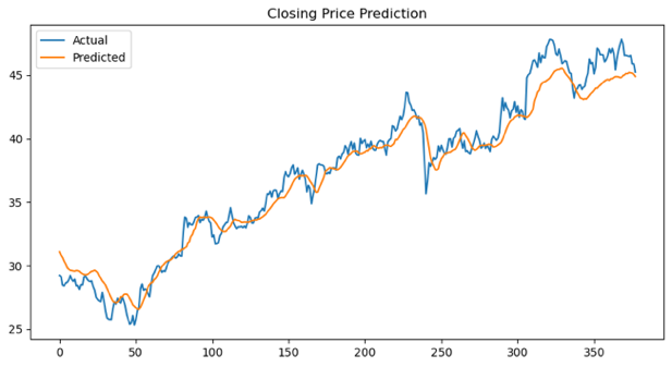
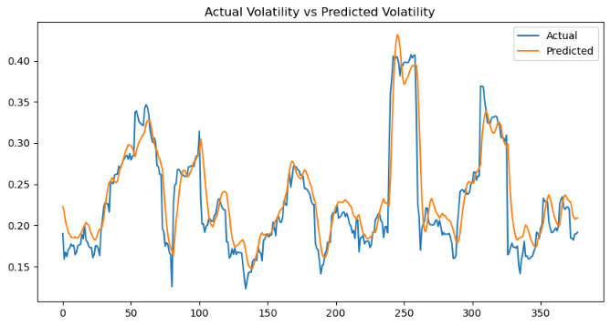
Considering the visual results (Figures 3–5), the predictions closely follow the actual trends in the test set, despite deviations in precise values. This alignment suggests that the MTL model can effectively captures the underlying patterns, though the inherent complexity and noise in stock time series data make exact challenges. The observed discrepancies may stem from sudden market fluctuations or the nonlinear dynamics of financial data, which are difficult to fully model. However, the MTL model’s ability to approximate the overall trends highlights its robustness and utility.

5. Discussion

5.1. Result Analysis

The MTL model consistently outperforms benchmark models across all tasks, demonstrating its ability to leverage shared information across related tasks to improve prediction accuracy. Classic ARIMA models perform poorly, especially in volume and volatility prediction, due to their inability to handle data with nonlinear dynamics and sudden spikes and drops, highlighting the limitations in capturing complex and nonlinear patterns in financial data. The DL models perform significantly better than ARIMA but worse than MTL, reflecting its better ability for processing time series data but the limitations in capturing related factors and information. These findings underscore the effectiveness of MTL for financial times series forecasting, particularly when tasks are interrelated.

5.2. Limitations

Regarding the MTL model in this experiment, while the performance has been improved for the volume prediction task, it still incurs a large percentage error due to the extreme spikes in trading volume data. Additionally, though the MTL model can learn efficiently by leveraging correlated information compared to single-task models, it faces some challenges due to its multi-task framework. Firstly, there may have situations where tasks have conflicting objectives or gradients, improving one task's performance can degrade the performance of others. This can lead to promising forecasts for only a subset of tasks. Secondly, the tasks may have various difficulty and complexity levels, and the MTL model will prioritize the easier tasks at the expense of the others. Those harder tasks cannot get enough attention and produce poor performance. Another obstacle is to determine optimal weights for task losses, unreasonable weights can lead to imbalanced and poor performance across the tasks.

6. Conclusion

This paper proposes a multi-task learning model (MTL) based on a CNN-LSTM-Attention architecture for simultaneously forecasting stock closing price, trading volume, and volatility. By incorporating technical indicators and leveraging shared information across tasks, the MTL model achieves significant improvements over the ARIMA and DL models. Future work may focus on further enhancing the performance, particularly the trading volume forecasting, by either incorporating external factors (e.g., market sentiment, economic indicators) or refining the model framework by exploring advanced architectures and loss-weighting strategies for better generalization. Additionally, future work can study more on resolving task conflicts and balancing task complexities to further improve MTL performance.

References

[1]. Sen, J., & Chaudhuri, T. D. (2017, April 25). A time series Analysis-Based Forecasting Framework for the Indian Healthcare sector. arXiv.org. https://arxiv.org/abs/1705.01144
[2]. Helli, S. S., Tanberk, S., & Demir, O. (2022). Forecasting Energy Consumption Using Deep Learning in Smart Cities. IEEE, 1–6. https://doi.org/10.1109/icaiot57170.2022.10121846
[3]. Hoseinzade, E., & Haratizadeh, S. (2019). CNNpred: CNN-based stock market prediction using a diverse set of variables. Expert Systems With Applications, 129, 273–285. https://doi.org/10.1016/j.eswa.2019.03.029
[4]. Mondal, P., Shit, L., & Goswami, S. (2014). Study of Effectiveness of Time Series Modeling (ARIMA) in forecasting stock Prices. International Journal of Computer Science Engineering and Applications, 4(2), 13–29. https://doi.org/10.5121/ijcsea.2014.4202
[5]. Petrică, A., Stancu, S., & Tindeche, A. (2016). Limitation of ARIMA models in financial and monetary economics. DOAJ (DOAJ: Directory of Open Access Journals). https://doaj.org/article/3b26dede3d584d9f8d3e52e0d0c5ae6e
[6]. Vasudevan, R. D., & Vetrivel, S. C. (2016). Forecasting Stock Market Volatility using GARCH Models: Evidence from the Indian Stock Market. Asian Journal of Research in Social Sciences and Humanities, 6(8), 1565. https://doi.org/10.5958/2249-7315.2016.00694.8
[7]. Siami-Namini, S., Tavakoli, N., & Namin, A. S. (2019, November 21). A comparative analysis of forecasting financial time series using ARIMA, LSTM, and BILSTM. arXiv.org. http://arxiv.org/abs/1911.09512
[8]. Büyükşahin, Ü. Ç., & Ertekin, Ş. (2019). Improving forecasting accuracy of time series data using a new ARIMA-ANN hybrid method and empirical mode decomposition. Neurocomputing, 361, 151–163. https://doi.org/10.1016/j.neucom.2019.05.099
[9]. Mei, W., Xu, P., Liu, R., Liu, J., & School of Management Science and Engineering Nanjing University of Finance and Economics. (2018). Stock price prediction based on ARIMA - SVM model. In 2018 International Conference on Big Data and Artificial Intelligence (ICBDAI 2018) [Conference-proceeding]. Francis Academic Press. https://doi.org/10.25236/icbdai.2018.00849
[10]. Ranjan, R., Patel, V. M., & Chellappa, R. (2017). HyperFace: a deep Multi-Task learning framework for face detection, landmark localization, pose estimation, and gender recognition. IEEE Transactions on Pattern Analysis and Machine Intelligence, 41(1), 121–135. https://doi.org/10.1109/tpami.2017.2781233
[11]. Samala, R. K., Chan, H., Hadjiiski, L. M., Helvie, M. A., Richter, C., & Cha, K. H. (2018). Cross-domain and multi-task transfer learning of deep convolutional neural network for breast cancer diagnosis in digital breast tomosynthesis. Medical Imaging 2018: Computer-Aided Diagnosis, 25. https://doi.org/10.1117/12.2293412
[12]. Ma, T., & Tan, Y. (2020). Multiple Stock Time Series Jointly Forecasting with Multi-Task Learning. 2022 International Joint Conference on Neural Networks (IJCNN), 1–8. https://doi.org/10.1109/ijcnn48605.2020.9207543
[13]. Yuan, C., Ma, X., Wang, H., Zhang, C., & Li, X. (2023). COVID19-MLSF: A multi-task learning-based stock market forecasting framework during the COVID-19 pandemic. Expert Systems With Applications, 217, 119549. https://doi.org/10.1016/j.eswa.2023.119549
[14]. Geurts, M., Box, G. E. P., & Jenkins, G. M. (2015). Time Series Analysis: Forecasting and Control (5th Ed.) https://doi.org/10.2307/3150485
[15]. Hyndman, R. J., & Athanasopoulos, G. (2013). Forecasting: principles and practice.
[16]. LeCun, Y., Bengio, Y., & Hinton, G. (2015). Deep learning. Nature, 521(7553), 436–444. https://doi.org/10.1038/nature14539
[17]. Dive into Deep Learning — Dive into Deep Learning 1.0.3 documentation. (n.d.). https://d2l.ai/
[18]. Gers, F. A., Schmidhuber, J., & Cummins, F. (2000). Learning to Forget: Continual Prediction with LSTM. Neural Computation, 12(10), 2451–2471. https://doi.org/10.1162/089976600300015015
[19]. Zhang, Y., & Yang, Q. (2017). An overview of multi-task learning. National Science Review, 5(1), 30–43. https://doi.org/10.1093/nsr/nwx105
[20]. Ruder, S. (2017, June 15). An overview of Multi-Task learning in deep neural networks. arXiv.org. https://arxiv.org/abs/1706.05098
Cite this article
Jiang,X. (2025). A Multi-Task Learning Model for Stock Market Forecasting. Applied and Computational Engineering,146,1-8.
Data availability
The datasets used and/or analyzed during the current study will be available from the authors upon reasonable request.
Disclaimer/Publisher's Note
The statements, opinions and data contained in all publications are solely those of the individual author(s) and contributor(s) and not of EWA Publishing and/or the editor(s). EWA Publishing and/or the editor(s) disclaim responsibility for any injury to people or property resulting from any ideas, methods, instructions or products referred to in the content.
About volume
Volume title: Proceedings of SEML 2025 Symposium: Machine Learning Theory and Applications
© 2024 by the author(s). Licensee EWA Publishing, Oxford, UK. This article is an open access article distributed under the terms and
conditions of the Creative Commons Attribution (CC BY) license. Authors who
publish this series agree to the following terms:
1. Authors retain copyright and grant the series right of first publication with the work simultaneously licensed under a Creative Commons
Attribution License that allows others to share the work with an acknowledgment of the work's authorship and initial publication in this
series.
2. Authors are able to enter into separate, additional contractual arrangements for the non-exclusive distribution of the series's published
version of the work (e.g., post it to an institutional repository or publish it in a book), with an acknowledgment of its initial
publication in this series.
3. Authors are permitted and encouraged to post their work online (e.g., in institutional repositories or on their website) prior to and
during the submission process, as it can lead to productive exchanges, as well as earlier and greater citation of published work (See
Open access policy for details).