1. Introduction

Artificial Intelligence (AI) has become a vital tool across people’s life and work, revolutionizing industries with its ability to learn from data. The ability of learning from data relies heavily on optimization algorithms. Among these, descent algorithms iteratively adjust weights and other parameters in neural networks based on gradient information. These algorithms are used to minimize the loss function, which measures the difference between optimal value and the actual value. By minimizing the loss, descent algorithm helps the AI model improve its ability to make accurate predictions. Mathematically, like M-estimator (a maximum-likelihood estimation) [1], given a dataset D and a model parameterized by θ, the goal is to solve:

\( {θ^{*}}=arg{\underset{θ}{min}{L}}(θ,D) \)

where L (θ, D) is the loss function. The descent algorithm iteratively updates θ using gradients of L.

Variants such as Stochastic Gradient Descent (SGD) offer additional improvements by refining the optimization process and allowing models to converge more efficiently.

1.1. Mathematical Challenges and Research Directions

In the optimization of descent algorithms for AI learning, several mathematical challenges arise that require ongoing research to address. One key issue is ensuring the convergence of optimization algorithms, particularly in the context of complex, non-convex loss landscapes [2]. In non-convex problems, the optimization process may get stuck in local minima or saddle points, which makes it difficult to find global solutions. Research into techniques such as saddle point avoidance and escape mechanisms continue to explore how to overcome these challenges.

Another important mathematical aspect is the design of efficient convergence rates. Under- standing and deriving convergence rates for descent algorithms under different conditions—such as with varying step sizes and complex neural network architectures—remains an open area of re- search. Moreover, the role of regularization in optimization is a critical subject, as it helps prevent overfitting by controlling the complexity of the model. Research into the optimal balance between model complexity and generalization performance is an ongoing effort.

In general, the mathematical foundations of AI optimization offer numerous research directions, from improving algorithmic efficiency to deepening the theoretical understanding of how different models converge during training.

2. Foundations of Descent Algorithms

Descent algorithms are a fundamental class of optimization techniques widely used in machine learning and artificial intelligence. These algorithms iteratively update model parameters, guiding the system towards an optimal solution. The most common method, gradient descent, relies on the gradient of the loss function to determine the direction of updates. In the following section, the article will explore the mathematical foundations of descent algorithms.

2.1. Dynamical Systems and Descent Algorithms

Gradient descent can be understood as a discrete dynamical system where the model parameters evolve over time in response to the gradient of the loss function [3]. In this view, each iteration represents a “step” in a time series. This process can be seen as a dynamical system with discrete time, where the parameters are adjusted at each time step according to a fixed rule. The dynamical system perspective allows us to analyze the trajectory of the algorithm’s parameter updates over time, determining whether the system converges to a stable point (i.e., the optimal solution) or oscillates or diverges. In particular, the stability of this system depends on the learning rate η, as an overly large step size can cause the system to “jump” away from the optimal point, while a very small step size can lead to slow convergence.

2.2. Gradient Descent and Extending Algorithms for Wider Situations

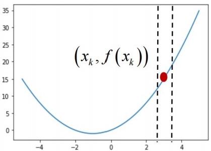
Figure 1: Visualization of gradient descent, retrieved from: https://bohrium.dp.tech/courses/5963419225/content?file=8570

Gradient descent is the most basic method of optimization, suggesting the fundamental principle of descent algorithm mathematically [4]. The method can be expressed as:

\( {θ_{t+1}}={θ_{t}}-η{∇_{θ}}L({θ_{t}}) \)

where:

\( {θ_{t}} \) represents the parameters of the model at iteration t, namely the red point on figure 1.

\( η \) represents the learning rate, controlling how much to adjust the parameters, namely how much the red point moves in one step.

\( {∇_{θ}}L({θ_{t}}) \) represents the derivation of the loss function with respect to the parameters, determining the direction and size of one step.

In practical problems, the derivation can be replaced by differences. There is no essential dis- tinction between the two, because they both use the idea of monotonicity.

\( Difference=\underset{Δ→0}{lim}{\frac{f({x_{k}}+{Δ_{2}})-f({x_{k}}-{Δ_{1}})}{({x_{k}}+{Δ_{2}})-({x_{k}}-{Δ_{1}})}} \)

\( derivation=\frac{df({x_{k}})}{dx}=\underset{Δ→0}{lim}{\frac{f({x_{k}}+Δ)-f({x_{k}})}{Δ}} \)

For convex optimization, gradient descent guarantees convergence to the global minimum under appropriate conditions, provided that the loss function is differentiable, and the learning rate is suitably chosen [5]. The update rule for gradient descent ensures that the parameters are consistently adjusted in the direction of the negative gradient, and each step brings the algorithm closer to a minimum.

Further discussions on convergence analysis and the mathematical complexities of these algorithms, including how they behave in different optimization landscapes, will be explored in discussion section.

2.3. Theoretical Limitations of First-Order Methods

Despite its widespread use, first-order methods like gradient descent have several theoretical limitations. One major challenge is their lack of second-order information about the curvature of the loss function. Gradient descent only uses the first derivative (the gradient), which can lead to inefficiencies when the loss function has regions with sharp curvatures or flat areas. In such cases, the algorithm may either overshoot the minimum or move too slowly, failing to exploit the structure of the problem effectively. The absence of second-order information means that gradient descent can perform poorly in situations where the loss function has steep and shallow regions, which require different step sizes for efficient progress.

Additionally, gradient descent is generally limited to local optimization and may converge to a local minimum, especially in non-convex optimization problems. While methods like simulated annealing can potentially escape these local minima by accepting worse solutions, gradient descent is deterministic and will typically settle into the nearest local minimum. This is a significant is- sue for problems with complex, multi-modal loss landscapes, such as those encountered in deep learning. To address these limitations, researchers have developed more advanced methods, such as second-order methods (e.g., Newton’s method), which use both first and second derivatives of the loss function to more efficiently navigate complex optimization surfaces.

3. Discussion

3.1. Convergence Analysis of Descent Algorithms

The convergence of descent algorithms in artificial intelligence depends on the properties of the objective function and the specific algorithmic framework. For any two points on the graph of a function, the line segment connecting them lies entirely above the graph – the function is called a convex function, as figure 2 shown, which means it has a single global minimum point. Mentioned previously, descent algorithm can solve optimization problem for convex function very easily. However, in non-convex settings, convergence is generally to a stationary point, which may be a local minimum or a saddle point. Special techniques are required to prevent these situations.

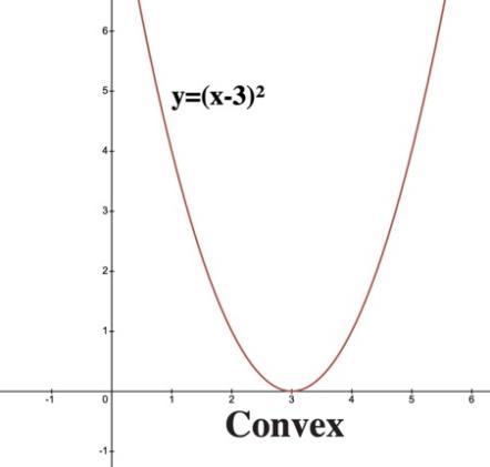
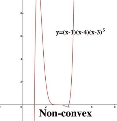
Figure 2: Comparison between convex function and non-convex function in 2-dimensional space

3.2. Methods to prevent local minima and minimax

To prevent descent algorithms from getting trapped in saddle points, several methods have been developed, each addressing different aspects of the optimization process.

3.3. Leveraging Strict Saddle Property

Strict Saddle Property is a key feature of minimax in non-convex optimization, which states the hessian matrix of every saddle point of a function has at least one negative eigenvalue [6]. Roughly speaking, saddle points exhibit at least one direction of negative curvature. This negative curvature allows second-order methods (such as Newton’s method) to escape these saddle points and continue towards a true local minimum or global optimum.

3.4. Perturbation Methods

Perturbation Methods is effective for escaping saddle points [7]. They introduce randomness or perturbations to the algorithm’s updates, which can prevent the optimization process from stagnating at a saddle point.

Stochastic Gradient Descent (SGD) is a gradient-based method widely used in machine learning [8][9]. As its name suggested, it is very similar with gradient descent (GD), which is elaborated previously. The only difference between them: SGD uses only a data point (or a mini-batch) of training set to update a parameter in one iteration or step, while GD runs through all samples in training set to update a parameter in one iteration. SGD takes much less time than GD when training set is very large. The analysis through time complexity is shown in following text.

Dataset size: Assume the dataset consists of N data points, each with D features.

Number of iterations(T): In SGD, the algorithm processes one data point per iteration, and it takes N iterations to go through the entire dataset once. Typically, SGD is used for many epochs, so the total number of iterations T can be much larger than N

So, the total time complexity for SGD and GD is: \( O(T\cdot N\cdot D) \)

While these seem similar to each other, the key difference is that SGD processes only one data point at a time, meaning the computational cost per iteration is significantly lower than the cost of processing the entire dataset in GD, which is

\( O(D)≤O(N\cdot D), for N \gt 1 \) ,

\( O(D)≪O(N\cdot D), when N≫1 \)

where O(D) represents the time complexity per iteration of SGD, O(N⋅D) represents the time complexity per iteration of GD.

The randomness in SGD, due to mini-batch updates, can help escape some local minima or saddle points to a degree. However, it doesn’t have an explicit mechanism to ensure global exploration of the solution space like Simulated Annealing (SA) does. Therefore, while it can sometimes escape shallow local minima, it may still end up stuck in deeper ones, especially in highly non-convex landscapes.

Simulated Annealing (SA) begins by initializing with a solution x₀ and an initial temperature T₀ [10]. At each iteration, the temperature is reduced according to the formula

T (t+1) = α T(t)

where 0<α<1 is the cooling factor. A neighbouring solution x′ is then generated by modifying the current solution x. The new solution x′ is accepted with a probability given by:

P \( (accept)=\begin{cases} \begin{array}{c} 1, if f({x^{ \prime }}) \lt f(x) \\ {e^{-\frac{-f({x^{ \prime }})-f(x)}{T}}}, if f({x^{ \prime }})≥f(x) \end{array} \end{cases} \)

where f(x) is the objective function value. The algorithm repeats this process, iterating through neighbour generation and acceptance, until the solution stabilizes, indicating the end of the process. To ensure convergence to the global minimum, the cooling schedule must be carefully controlled. At the beginning, the high temperature lets the system to explore a wide range of solutions, including accepting worse solutions that help avoid local minima. As the temperature decreases, the algorithm becomes more selective, favouring better solutions and eventually settling in a local minimum. If the cooling is slow enough, simulated annealing is theoretically guaranteed to find the global minimum in the limit, given infinite time, due to its connection with the Boltzmann distribution, which dictates that the probability of accepting a worse solution decreases as the temperature lowers.

Together, these methods offer a robust framework for optimizing non-convex functions, preventing descent algorithms from being trapped in local minima or saddle points, and enabling them to find better solutions more efficiently.

3.5. Evaluating Descent Algorithms

When evaluating descent algorithms, two key aspects is often considered: asymptotic convergence and finite-time convergence. These two methods assess the behaviours of optimization algorithms, particularly how they approach the minimum of an objective function over time. In this context, convergence refers to the algorithm’s ability to minimize the objective function as the number of iterations increases. Asymptotic convergence focuses on the long-term behaviour of an algorithm, describing how the algorithm behaves as the number of iterations, t, becomes large [11]. More formally, the algorithm is said to converge asymptotically if the parameters \( θ \) _t of the model converge to the optimal solution θ^∗ as t → ∞, such that:

\( \underset{t→∞}{lim}{{θ_{t}}}={θ^{*}}. \)

In this case, the objective function f (θ) approaches its minimum value f(θ*) as the algorithm proceeds. For many gradient-based methods, the learning rate η approaches zero, the gradient of the objective function at the iterate also approaches zero, suggesting convergence to a minimum.

\( \underset{η→0}{lim}{|}∇f({x_{t}})|=0 \)

A common theoretical result that guarantees asymptotic convergence is provided by the gradient descent method, which, under certain conditions (e.g. convexity of f), converges to the global minimum as t→∞. For a convex function f, the convergence rate is often analysed in terms of distance to optimality \( {d_{t}}=|{θ_{t}}-{θ^{*}}| \) ,which typically follows a relationship like:

\(  {d_{t+1}}≤ρ{d_{t}}, where 0 \lt ρ \lt 1. \)

This implies that the distance between the current solution and the optimal solution decreases exponentially with each iteration, where ρ is a constant depending on the properties of f and the learning rate η.

3.6. Finite-time Convergence

Asymptotic convergence evaluates the long-term behaviours of an optimization algorithm. Finite-time convergence focuses on its performance within a limited number of iterations. Compared to asymptotic convergence, finite-time convergence examines the convergence rate over a finite number of steps, often measured by convergence rates such as linear, sublinear, and superlinear convergence [12].

Linear convergence is featured by an exponential decrease in the objective function value f (θ_t) at iteration t. Specifically, the difference between the current function value and the optimal value f (θ*) decreases by a constant fraction at each step. Mathematically, this is expressed as:

\( f({θ_{t+1}})-f({θ^{*}})≤α(f({θ_{t}})-f({θ^{*}})), 0 \lt α \lt 1. \)

Here, α is the convergence rate constant. Linear convergence implies that the number of iterations required to achieve a small error grows relatively slowly, making it a desirable property for many optimization algorithms.

Compared to linear convergence, Sublinear convergence has a slower rate, typically on the order of O(1/t). In other words, the algorithm gets closer to the optimal solution at a diminishing rate over time. For example:

\( f({θ_{t}})-f({θ^{*}})≤\frac{C}{t}, \)

where C is a constant. Sublinear convergence is common in scenarios where the algorithm is not optimally tuned, or the problem is ill-conditioned. This kind of rate is easily to see in gradient descent methods with fixed step.

Furthermore, superlinear convergence is a faster form of convergence where the rate of improvement increases dramatically as the algorithm approaches the optimal solution. A classic example is Newton's method, which exhibits quadratic convergence [13]. This can be expressed as:

\( {d_{t+1}}≤βd_{t}^{2}, for some constant β \gt 0, \)

where d_t​ represents the distance to the optimal solution at iteration t. Superlinear convergence implies that the error decreases very quickly as the algorithm gets closer to the optimal point, making it highly efficient for well-conditioned problems. In summary, the evaluation of descent algorithms through Asymptotic and Finite-Time Convergence provides a comprehensive understanding of their efficiency. Asymptotic convergence focuses on the ultimate destination. On the other hand, finite-time convergence measures how quickly an algorithm reaches a solution within a finite number of iterations, with different convergence rates dictating how rapidly the objective function value decreases. Depending on the problem and the algorithm used, both types of convergence are critical in determining the effectiveness of a descent method in practice.

4. Conclusion

This article gives mathematical insight into aspects of descent algorithms, while having limitations and allowing for further exploration in research. The main issue stems from the implementation of these algorithms, where certain assumptions made during the theoretical analysis do not generally transfer into practical applications. For example, these assumptions of linear convergence or saddle point escape, or the idealized case of having a smooth optimization landscape may be hard to achieve in practice in real-world and complex noisy environments. As machine learning and artificial intelligence advance further, researchers require descent algorithms that not only work mathematically but also translate well in practice against these challenges. This research, looking at nature alone without these complexities, is a useful stepping stone toward future large-scaled studies that include these features.

While research continues, it is important to think not only about the mathematical and computational performance of these algorithms but additionally on their effect in society. Descent algorithms are popular for practical applications in natural language processing, computer vision, autonomous actuation systems, etc. ,all of which often have ethical issues. So now, as AI technologies keep developing, researchers, practitioners, and policymakers, need to collaborate with one another to ensure that such platforms are used responsibly, and are designed with fairness, transparency, and accountability in mind.

References

[1]. Wikipedia Contributors. (2024, November 5). M-estimator. Wikipedia; Wikimedia Foundation. https://en.wikipedia.org/wiki/M-estimator
[2]. Jain, P., & Kar, P. (2017). Non-convex Optimization for Machine Learning. Foundations and Trends® in Machine Learning, 10(3-4), 142–336. https://doi.org/10.1561/2200000058
[3]. Baldi, P. (1995). Gradient descent learning algorithm overview: a general dynamical systems perspective. IEEE Transactions on Neural Networks, 6(1), 182–195. https://doi.org/10.1109/72.363438
[4]. Suvrit Sra, Nowozin, S., & Wright, S. J. (2012). Optimization for machine learning. Mit Press.
[5]. Chatterjee, S. (2022). Convergence of gradient descent for deep neural networks. ArXiv (Cornell University). https://doi.org/10.48550/arxiv.2203.16462
[6]. Jin, C., Ge, R., Praneeth Netrapalli, Kakade, S. M., & Jordan, M. I. (2017). How to escape saddle points efficiently. International Conference on Machine Learning, 1724–1732.
[7]. Spall, J. C. (1999). Stochastic optimization and the simultaneous perturbation method. https://doi.org/10.1145/324138.324170
[8]. Ge, R., Huang, F., Jin, C., & Yang, Y. (2015). Escaping From Saddle Points --- Online Stochastic Gradient for Tensor Decomposition. ArXiv (Cornell University). https://doi.org/10.48550/arxiv.1503.02101
[9]. Kiefer, J., & Wolfowitz, J. (1952). Stochastic Estimation of the Maximum of a Regression Function. The Annals of Mathematical Statistics, 23(3), 462–466. http://www.jstor.org/stable/2236690
[10]. Kirkpatrick, S., Gelatt, C. D., & Vecchi, M. P. (1983). Optimization by Simulated Annealing. Science, 220(4598), 671–680. https://doi.org/10.1126/science.220.4598.671
[11]. Wah, B. W., Chen, Y., & Wang, T. (2006). Simulated annealing with asymptotic convergence for nonlinear constrained optimization. Journal of Global Optimization, 39(1), 1–37. https://doi.org/10.1007/s10898-006-9107-z
[12]. Axelsson, O., & Kaporin, I. (2000). On the sublinear and superlinear rate of convergence of conjugate gradient methods. Numerical Algorithms, 25, 1-22.
[13]. Drobny, S., & Weiland, T. (2000). Numerical calculation of nonlinear transient field problems with the Newton-Raphson method. IEEE Transactions on Magnetics, 36(4), 809–812. https://doi.org/10.1109/20.877568
Cite this article
Lyu,W. (2025). Mathematical Analysis of Descent Algorithms in Artificial Intelligence: Convergence, Loss Landscapes, and Structural Optimization. Applied and Computational Engineering,145,14-21.
Data availability
The datasets used and/or analyzed during the current study will be available from the authors upon reasonable request.
Disclaimer/Publisher's Note
The statements, opinions and data contained in all publications are solely those of the individual author(s) and contributor(s) and not of EWA Publishing and/or the editor(s). EWA Publishing and/or the editor(s) disclaim responsibility for any injury to people or property resulting from any ideas, methods, instructions or products referred to in the content.
About volume
Volume title: Proceedings of the 3rd International Conference on Software Engineering and Machine Learning
© 2024 by the author(s). Licensee EWA Publishing, Oxford, UK. This article is an open access article distributed under the terms and
conditions of the Creative Commons Attribution (CC BY) license. Authors who
publish this series agree to the following terms:
1. Authors retain copyright and grant the series right of first publication with the work simultaneously licensed under a Creative Commons
Attribution License that allows others to share the work with an acknowledgment of the work's authorship and initial publication in this
series.
2. Authors are able to enter into separate, additional contractual arrangements for the non-exclusive distribution of the series's published
version of the work (e.g., post it to an institutional repository or publish it in a book), with an acknowledgment of its initial
publication in this series.
3. Authors are permitted and encouraged to post their work online (e.g., in institutional repositories or on their website) prior to and
during the submission process, as it can lead to productive exchanges, as well as earlier and greater citation of published work (See
Open access policy for details).