1. Introduction

More than 280 million individuals of all ages (or around 3.5% of the world's population) suffer from depression, a mental condition characterized by low mood and aversion to activity [1,2]. The symptoms of depression, which are categorized medically as a mental and behavioral disorder [3], impact a person's thoughts, behavior, motivation, feelings, and sense of wellbeing. There was a paper used machine learning (ML) to study the kinds and differences of those methods. In order to find new materials with lower costs, shorter cycles, and higher efficiency, they used ML to help with material analysis and testing. In addition, they also summarized the mature areas of ML found in materials science, which brings great help to ML tasks [4]. There is also a paper that used ML in the field of fluid mechanics. They use ML to extract information from the data and turn it into useful knowledge about fluid mechanics. The use of ML in fluid mechanics is extensive, from past history to future opportunities, which are introduced in this paper. Also, they point out that ML has the potential to change the course of research and industrial applications [5]. ML also has great value in biology. One paper presented some successful cases of ML model in biotechnology application. They point out that ML has the potential to be used in the design of biosystems in the future [6]. By those papers above, it is easy to observe that ML has a lot of attributions in different fields on modeling. The goal of our paper is to predict the possibility of depression based on different features in the public dataset. The topic of our paper is Application of Machine Learning on Depression Analysis. Depression may can be caused many different reasons (e.g., age, incoming salary, number of children, married or not, education level, living expenses). The main job of this study is to predict whether the individuals have suffered the depression or not and to find which is the most influential features. The reason why the authors choose this topic is to hope that more people can understand, care, and help those with depression or depression tendencies. They are really in a very painful situation. The methods used are random forest, naive bayes, neutral network, SVM. For a range of data, random forest generates precise classifiers. It can manage many different input variables. When establishing categories, it can evaluate the significance of variables. As a probability-based classification method, Naive Bayes is widely used. In most cases, it has better classification prediction and faster training speed. SVM has three main benefits. First at all, SVM can efficiently handle the classification problem of high-dimensional feature space. Secondly, SVM saves memory well. Finally, the application of SVM is very wide. The Random Forest and Neural network had the best overall accuracy of 86.8%, according to the results as a whole. The authors also conduct analysis on exploiting the most important features by feature correlation, the authors find that the age and education level can mainly lead to depression. In the future, the main object is processing methods for the datasets and making improvement on Attention and treatment of depression.

2. Method

2.1. SVM

The basic model of the SVM [7,8], a binary classification model, is a linear classifier that is defined as the greatest interval on the feature space. In addition to kernel methods, SVM is essentially a nonlinear classifier. Character identification, facial recognition, pedestrian detection, text classification, and other application scenarios are some of the key classification problems that SVM is employed for. SVM is a supervised learning model used for pattern recognition, classification (outlier identification), and regression analysis in the field of machine learning. The fundamental idea behind SVM is to identify the separating hyperplane with the largest geometric interval and the ability to accurately split the training data set. The training process of SVM is to first obtain the Lagrangian function using the Lagrange multiplier method, and then use its duality by swapping the minimum and maximum positions to find its dual problem. For support vector machines, if the data points are in p dimension, the authors use a p-1-dimensional hyperplane to separate these points. A reasonable choice for the optimal hyperplane is the hyperplane that separates the two classes by the largest margin. Therefore, the SVM selects the hyperplane that maximizes the distance to the hyperplane for the data points closest to the hyperplane, which is shown in Figure 1.

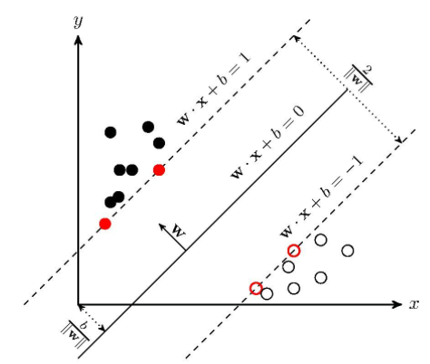
SVM has three main benefits. First at all, SVM can efficiently handle the classification problem of high-dimensional feature space. Secondly, SVM saves memory well. Finally, the application of SVM is very wide.

2.2. Naive Bayes

Naive Bayes [9,10] is a generative model that computes probabilities for classification and can be used for multi-classification problems and is suitable for incremental training. A Bayesian-based technique called naive Bayes makes the assumption that the feature conditions are unrelated to one another. The foundation of Naive Bayes is the idea of learning the joint probability distribution from input to output with a predetermined training set, presuming independence between feature terms. One acquires knowledge of the joint probability distribution from the input to the output. The input is then utilized to determine the output that maximizes the posterior probability based on the learned model. The advantages of Naive Bayes are that, firstly, its algorithm is logically simple and easy to implement. Secondly, it has low space-time overhead in the classification process. As a probability-based classification method, Naive Bayes is widely used. In most cases, it has better classification prediction and faster training speed.

2.3. Random Forest

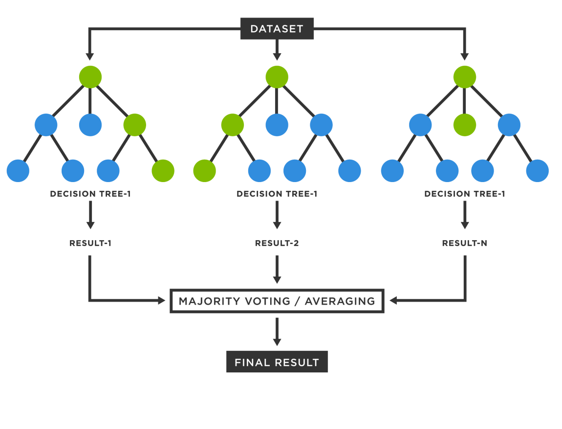
As shown in Figure 2, random forest is an integrated algorithm consisting of decision trees, in addition to the absence of any correlation between various decision trees. Each decision tree in the forest will evaluate and categorize each new input sample independently when performing a classification task. Each decision tree will then produce its own classification result, and the random forest will use the classification result that has the most classifications as the final outcome. As instances of where random forest is applied, consider the following four industries: banking, healthcare, the stock market, and e-commerce. Random Forest algorithms can be used in the banking industry to identify loyal consumers as well as fraudulent ones. Random Forest algorithms can be used in the medical profession to determine whether the various components of a drug are blended properly before usage and to diagnose illnesses by reviewing patient medical information. Random forest algorithms may be used to identify stocks that exhibit volatile behavior and forecast profits or losses in the stock market. Random forest algorithms may be used in e-commerce to foretell whether buyers would enjoy the products the system suggests based on their prior buying behavior. For a wide range of inputs, random forest generates precise classifiers. It can accommodate many different input variables. It may evaluate a variable's significance while establishing categories.

2.4. Neural Network

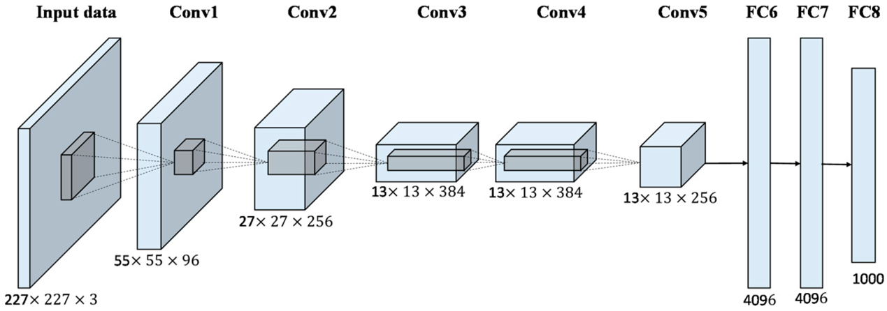
A mathematical or computer model called a neural network may be used to estimate or approximation a function by simulating the structure and operation of a biological neural network [11,12]. As shown in Figure 3, a neural network mainly consists of: an input layer, hidden layers, and an output layer. It is a complex network of neurons that function as simple fundamental components in an adaptive nonlinear dynamic system. Although individual neuron's structure and function are quite straightforward, the behavior of the entire system produced when several neurons are combined is extremely complicated. Several fundamental aspects of how the human brain functions are reflected in neural networks, which are just a type of imitation, simplification, and abstraction of biological systems rather than accurate representations. There are many uses for neural networks, but the three primary ones are in image and video (such as image identification and segmentation), medicine, and gaming (such as medical image diagnostics) (e.g. the invention of AlphaGO). First and foremost, distributed storage and fault tolerance are the major benefits of neural networks. Additionally, neural networks handle information quickly and efficiently in a large number of simultaneous, hierarchical units. Thirdly, neural networks are able to adapt to their surroundings and learn from outside sources. The reason neural networks can handle some issues with extremely complicated environmental input, hazy prior knowledge, and hazy inference rules is because they possess these traits. In our experiment, the architecture of CNN method contains 5 convolution layers and three fully-connected layers and then the results are provided.

3. Experiments

3.1. Dataset Description

The dataset the authors choose is depression from gaggle, its link is: https://www.kaggle.com/datasets/diegobabativa/depression. This dataset involves the analysis of depression, consisting of a study about life conditions of people who live in rural zones. The dataset contains 23 columns or dimension and a total of 1432 rows of objects: sex, age, family status, number of children, level of education, total number of family members, living costs, obtained asset, durable asset, saved asset, other expenses, incoming wage, incoming own farm, incoming business, incoming no business, farm expenses, employment, lengthy investigation, and no lengthy investigation. label 0 denotes the individuals do not suffer depression and label 1 calculates the persons in depression.

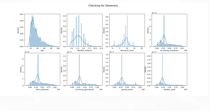
As shown in Figure 3, this group of graphs are used for checking the skewness of those different features.

The authors also plot the heat map, which showed that the depression is most relevant to age with 0.10 (positive relation), and the least relevant to education with -0.10 (negative relation).

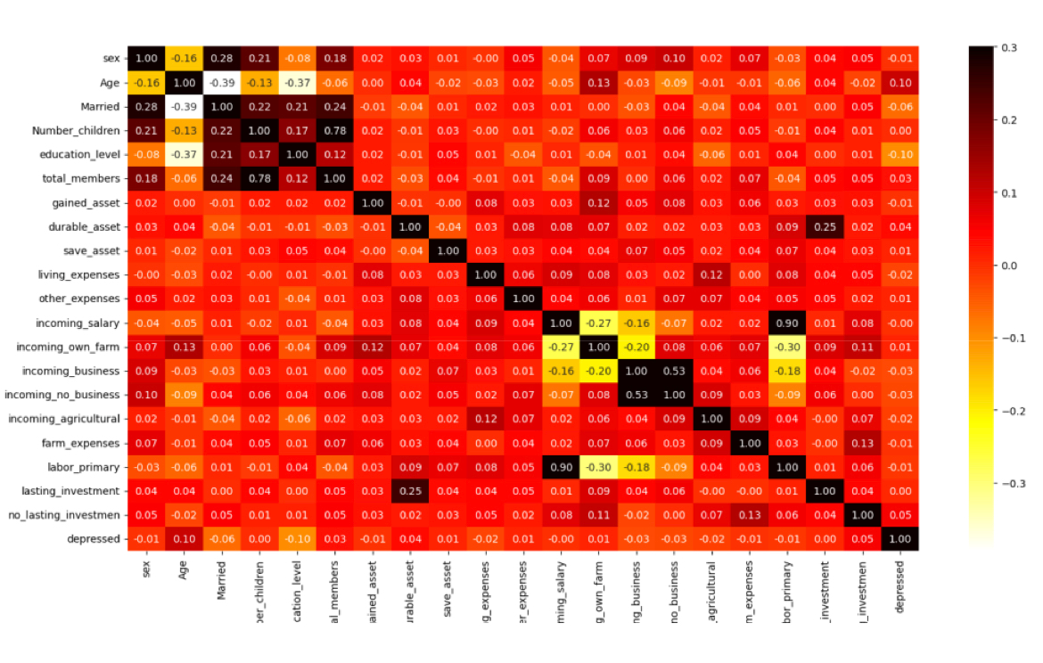
As shown in Figure 4, the third part of graphs the authors plot are bar charts which show the relationship between some features and depression. Finally, from Figure 4, the most influential factor among all is the age. The most common age of depression patients is between the ages of twenty and thirty. Ranking the second is educational level and living expenses, which are very difficult to change.

Table 1. Overall performance for the utilized methods.

The statistics of the utilized methods are listed in Table 1. Where both the Neural Network and Random Forest have the highest accuracy among all four methods. The best accuracy of those methods is 86.8%, while the SVM has the lowest accuracy, which is 74.1%. All the methods show reasonable performance, which can validate the effectiveness of machine learning based depression prediction.

4. Conclusion

In this paper, the authors aim to exploit the machine learning method into depression prediction task. Our approach uses the Navïe Bayes, Supported Vector Machine, Random Forest, and Neural Network four separate techniques. The outcomes show that among all the algorithms, Neural Network and Random Forest both produce the best outcomes. The best accuracy is 86.8%. Furthermore, the research find that the most influential feature is age and education level. The most common age for onset is between the ages of 20 and 30. On the basis of age, adding grown family factors will have a greater impact. The second influential set is education level and living expenses. These two factors come from family impact. These factors are really difficult to be change. Among the factors causing depression, there is not any internal factors, so it can be seen that depression is a 100 percent acquired disease. Also, gender doesn't have any effect on depression. The future works planned is to make some improvements on the processing methods for datasets that the authors are not perfect at current period. And also, the authors want to use data analysis to help us finding what is the best way to cure and ease depression. For example, seeing a psychiatrist, chatting with family members, chatting with friends, traveling, exercising, listening to music, etc. To sum up, with the results the authors got, people between the ages of 20 and 30 with high education level and more living expenses are more prone to depression. But it is not related to the gender at all.

References

[1]. "NIMH Depression Basics". www.nimh.nih.gov. 2016. Archived from the original on 11 June 2013. Retrieved 22 October 2020.
[2]. "Depression". www.who.int. Archived from the original on 26 December 2020. Retrieved 7 April 2021.
[3]. Sartorius N, Henderson AS, Strotzka H, Lipowski Z, Yu-cun S, You-xin X, et al. "The ICD-10 Classification of Mental and Behavioural Disorders Clinical descriptions and diagnostic guidelines" (PDF). www.who.int World Health Organization. pp. 30–1. Archived (PDF) from the original on 17 October 2004. Retrieved 23 June 2021
[4]. Wei, J., Chu, X., Sun, X. Y., Xu, K., Deng, H. X., Chen, J., ... & Lei, M. (2019). Machine learning in materials science. InfoMat, 1(3), 338-358.
[5]. Brunton, S. L., Noack, B. R., & Koumoutsakos, P. (2020). Machine learning for fluid mechanics. Annual review of fluid mechanics, 52, 477-508.
[6]. Volk, M. J., Lourentzou, I., Mishra, S., Vo, L. T., Zhai, C., & Zhao, H. (2020). Biosystems design by machine learning. ACS synthetic biology, 9(7), 1514-1533.
[7]. Noble, W. S. (2006). What is a support vector machine?. Nature biotechnology, 24(12), 1565-1567.
[8]. Suthaharan, S. (2016). Support vector machine. In Machine learning models and algorithms for big data classification (pp. 207-235). Springer, Boston, MA.
[9]. Rish, I. (2001, August). An empirical study of the naive Bayes classifier. In IJCAI 2001 workshop on empirical methods in artificial intelligence (Vol. 3, No. 22, pp. 41-46).
[10]. Leung, K. M. (2007). Naive bayesian classifier. Polytechnic University Department of Computer Science/Finance and Risk Engineering, 2007, 123-156.
[11]. Krizhevsky, A., Sutskever, I., & Hinton, G. E. (2012). Imagenet classification with deep convolutional neural networks. Advances in neural information processing systems, 25, 1097-1105.
[12]. Simonyan, K., & Zisserman, A. (2014). Very deep convolutional networks for large-scale image recognition. arXiv preprint arXiv:1409.1556.
Cite this article
Chen,W.;Fan,Y.;Zhou,J. (2023). Depression prediction using machine learning algorithms. Applied and Computational Engineering,5,379-385.
Data availability
The datasets used and/or analyzed during the current study will be available from the authors upon reasonable request.
Disclaimer/Publisher's Note
The statements, opinions and data contained in all publications are solely those of the individual author(s) and contributor(s) and not of EWA Publishing and/or the editor(s). EWA Publishing and/or the editor(s) disclaim responsibility for any injury to people or property resulting from any ideas, methods, instructions or products referred to in the content.
About volume
Volume title: Proceedings of the 3rd International Conference on Signal Processing and Machine Learning
© 2024 by the author(s). Licensee EWA Publishing, Oxford, UK. This article is an open access article distributed under the terms and
conditions of the Creative Commons Attribution (CC BY) license. Authors who
publish this series agree to the following terms:
1. Authors retain copyright and grant the series right of first publication with the work simultaneously licensed under a Creative Commons
Attribution License that allows others to share the work with an acknowledgment of the work's authorship and initial publication in this
series.
2. Authors are able to enter into separate, additional contractual arrangements for the non-exclusive distribution of the series's published
version of the work (e.g., post it to an institutional repository or publish it in a book), with an acknowledgment of its initial
publication in this series.
3. Authors are permitted and encouraged to post their work online (e.g., in institutional repositories or on their website) prior to and
during the submission process, as it can lead to productive exchanges, as well as earlier and greater citation of published work (See
Open access policy for details).