1. Introduction

Machine learning is a concept that lets machines learn from a certain set of data so that they can make decisions like humans do. The biggest difference between machine learning and traditional coding is that machine learning does not necessarily need to tell the computer the step-by-step procedure like traditional coding, whose instructions are mostly based on if-then structures. Machine learning is able to detect patterns in data and learn from them, and then give the desired output. With the evolution of machine learning and its algorithms, humans can now use them as a powerful tool to accomplish various tasks in all walks of life [1]. This paper will focus on the algorithms of machine learning, such as Linear Regression and Decision Trees. Machine learning algorithms are not the same as machine learning models. Algorithms in machine learning are the means to process the data set. The model of machine learning is an output of a machine learning algorithm runs on a data. Machine learning is able to process huge amounts of data [2]. However, there does not exist a single algorithm that is optimal for all kinds of data and problems, so it is crucial to take a detailed examination of machine learning algorithms [3]. Here are the algorithms based on the different types of machine learning. This paper will assist the reader in getting started with machine learning and laying the groundwork for future exploration into more advanced machine learning.

2. Supervised learning

A set of labeled data is necessary for supervised learning, in which case we will be certain of the object classifications. For problems like picture categorization, fraud detection, and spam filtering, supervised learning is appropriate [4]. Regression and classification are two categories of issues that might arise with supervised learning. In supervised learning, classification refers to the separation and classification of the data points. It will categorize and divide the entire sample into categories for simple interpretation. Regression analysis is a method for figuring out how a dependent variable and one or more independent variables are related. They can be applied to questions with continuous variables, such market movements or weather forecasts.

2.1. Support Vector Machine

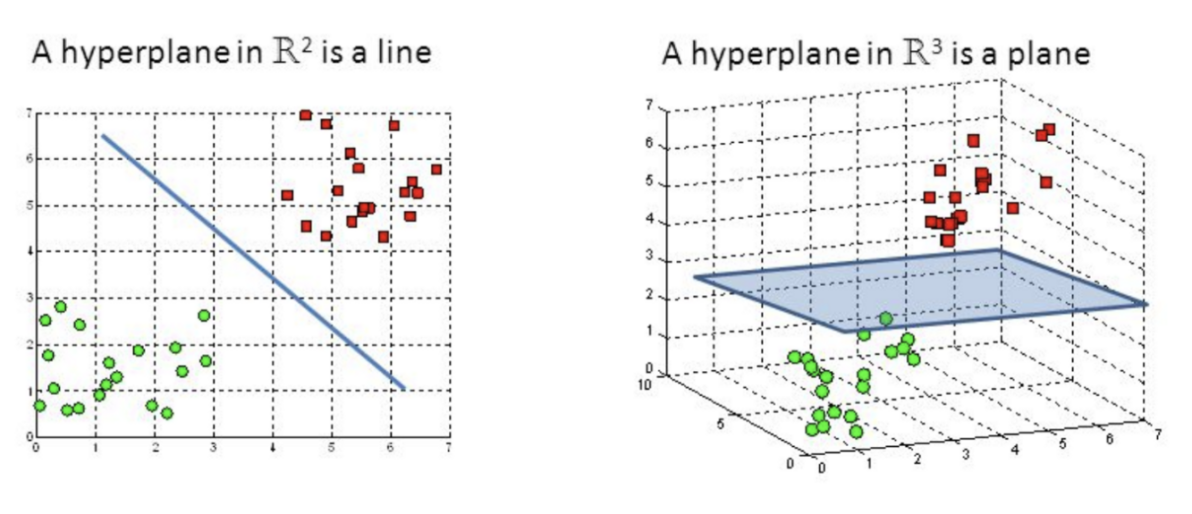
It is widely used in both classification and regression, but it is mostly used for classification. Support Vector Machine, as shown in Figure 1, is an algorithm that finds a hyperplane in an N dimensional space that can distinctly classify the objects with N number of features. There are infinite number of possible hyperplanes that can separate the data points, but it needs to be optimized for the hyperplane with the biggest margin. The margin is the distance between the closest different data points. With the largest margin possible, the future data being predicted will have more confidence for the classification.

2.2. Naive Bayes

Naïve Bayes classifier is probabilistic classifier based on the Bayes Theorem of probability, which is given as

P(A|B) = P(B|A) * P(A) / P(B)

In Naïve Bayes, it assumes that a specific feature of a class is not related to the presence of other features, and then it will achieve classification purpose depending on the conditional probability. Naïve Bayes is suitable for problems like classifications. For example, if an object can be round, green, and is a fruit, it might be a watermelon. This classification is based on the fact that these features do not affect each other, which makes Naïve Bayes a good choice of algorithm.

2.3. Decision Tree

Decision tree is a method that is used to classify a given object by answering a series of simple questions. Figure 2 indicates a general pattern of a decision tree. The root node of the tree is the input data pattern, and the leaf nodes are the categories that can be filtered through and then achieve the correct output [5]. Its structure is like a flow chart, it classifies the input data step by step. It is easy to understand and interpret because it is very close to human decision-making. However, it might turn out to be overfitting if the tree depth is too great [6].

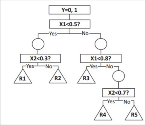
The Decision Tree algorithm can be described as three steps: first, determine the root node; second, calculate the entropy of the class and each attribute after splitting. Then, calculate the information gain of each split, which is the difference between the entropy of the previous step and use the highest one to create a child node until the information gain is small enough. After that, perform further splitting and pruning to adjust the model to avoid over-fitting.

2.4. K-Nearest Neighbor

K-Nearest Neighbor is a classification algorithm that is based on the Euclidean distance between the test samples and the training sample[7]. KNN can be performed when the sample data distribution is unknown because of its feature of measuring the geometric distance. K is the number of the closest neighbors that the unsorted data point has. For example, if K=4, after calculating the Euclidean distance between the unsorted data point and every other point, find the smallest four distances, and whichever category has the most smallest distances will the new data point go to. This core feature of KNN makes it possible that it fits any kind of data and suitable for both classification and regression. However, it is computationally expensive because it needs to store all the data and calculate through all the data, and it takes up more memory space to store all the training data.

2.5. Linear Regression

Linear Regression is an algorithm to find the best linear relation to fit for a model, which has to be a line. It is easy to implement and has less complexity compared to other algorithms, but can be badly affected by outliers and oversimplifies the real-world problem, so it is not recommended to use for actual problems.

The equation of a simple linear regression between two variables can be given as: y= a0+a1x+ ε, where y is the dependent variable and x is the dependent variable. It is our job to determine the a0 and a1, which is the intercept of the line and the linear regression coefficient, and ε is the random error. The most common application of linear regression is to evaluate trends and make estimations. For example, it can be used in business analysis to make predictions on a company’s annual revenue based on previous years.

3. Unsupervised learning

3.1. K-Means Clustering

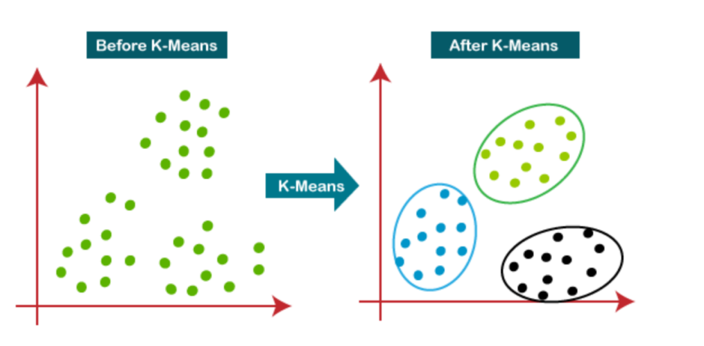
K-mean is an unsupervised learning algorithm that clusters the unlabeled data into labeled data without being given the correct answer like in supervised learning [8]. K is the number of clusters that needs to be predefined so that the process will separate the data into K number of clusters. There are two tasks the K-mean algorithm will perform. Firstly, do an iterative process to find the best K center points or centroids. Then, assign each data points to the closest k-center or centroid, creating K number of clusters. After this algorithm is performed, each cluster will have their own sorted data points that have commonalities, and they are far from other clusters. However, it might be difficult to predict the value of K at the beginning, and the output will change significantly if the K value is changed.

3.2. Principal Component Analysis

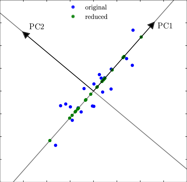
PCA is a way to reduce the dimension of the data by projecting it onto lines in lower dimensions, which are called the principal components. The first principal component starts in the direction of the greatest variance, which is calculated by finding eigenvalues of the covariance matrix of the data. PCA helps to interpret the data while maintaining the important features as much as possible. As shown in Figure 4, the blue points are the original points and the green points are the reduced dimension points where two dimensional data is reduced to one dimensional. PC1 and PC2 are orthogonal to each other, and here we see that PC1 is the better fit for the original data than PC2. The difference between PCA and Linear regression is that PCA reduces the dimension while linear regression keeps the original dimension of the data.

4. Reinforcement learning

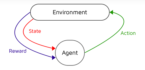
Reinforced learning is about how an intelligent agent would act in a certain environment to get the maximized the cumulative reward [9]. The intelligent agent here refers to a program that can make decisions or perform tasks. Figure 5 gives the general steps of reinforcement learning. Reinforcement learning usually consists of the following steps. The agent first observes the input state before choosing an action using a decision-making function, also referred to as a policy. The action and reward are recorded once the agent completes the task and receives the reinforcement or reward from the surrounding area. This process continues so that it keeps reinforcing itself. Here are some reinforcement learning algorithms.

4.1. Markov Chain and Markov Decision Process

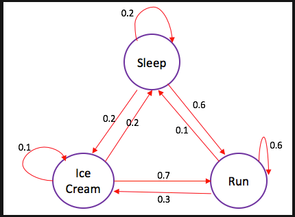
Reinforcement learning’ process can be described as a Markov Chain. A Markov Chain describes a process with a finite number of states where the transition between them is substantially dependent on its immediate previous state. For example, games like Snake and Ladder, where the movement is primarily based on the number of dice, is a Markov Chain. Meanwhile, card games like blackjack are not a Markov Chain, because the action takes more consideration of previous cards, which is the memory. Figure 6 is a graph of a Markov Chain. In reinforcement learning, a Markov Decision Process is used to determine the intelligent agent’s decision upon the environment. The transition between the states is called Markov Transition.

4.2. Monte Carlo method

Monte Carlo method is a method to simulate the probability with frequency. It relies on repeat random sampling to obtain numerical results that might be deterministic in principle [10]. A classic example of Monte Carlo method is to estimate the pi. Having a square and a circle cut to the edges of it and drop random point inside the square. The probability of a point dropped inside the circle would be the area of the circle divided by the area of the square, which is pi/4. Now if we throw enough number of random points into the square, we can see the frequency of points that falls into the circle to get as probability, which gives us the estimated value of pi. Monte Carlo method is widely used in many areas, here in reinforcement learning, it is helpful to get the probability distribution of transition between states [11].

5. Neural Network and Deep Learning

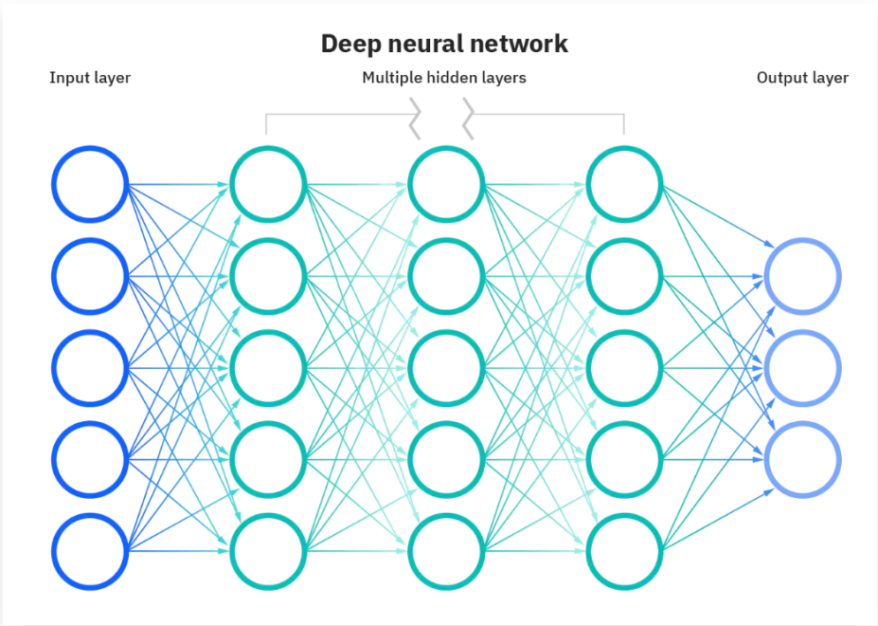
Neural networks make up the backbone of deep learning [12], which has three layers: the input layer, output layer, and the hidden layer in the middle. The depth of the multiple hidden layers gives the name to deep learning algorithms. Figure 7 is a graph of a neural network with multiple hidden layers. Considering the neural network in whole, its function is to get input and spit output. Therefore, a neural network can be used to approximate the state-value function, which is the policy part in reinforcement learning. That is, neural networks can guide the intelligent agent to make transitions to the next state in reinforcement learning.

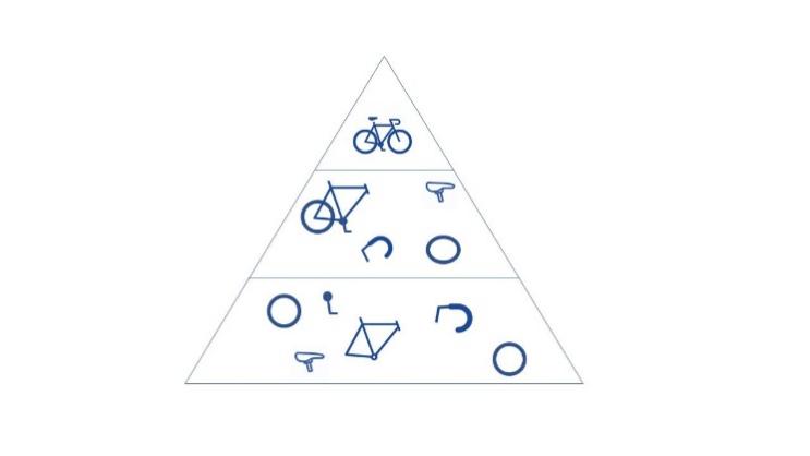
Convolutional neural network(CNN) is widely used in the application of neural network in classification and computer vision tasks. In general, CNN enables neural networks to break down and extract key features of the input [13]. For example, in Figure 8, if the input is an image of a bicycle, it will finally identify its features like the handle, wheel, and frame. It will then go lower-pattern of the features.

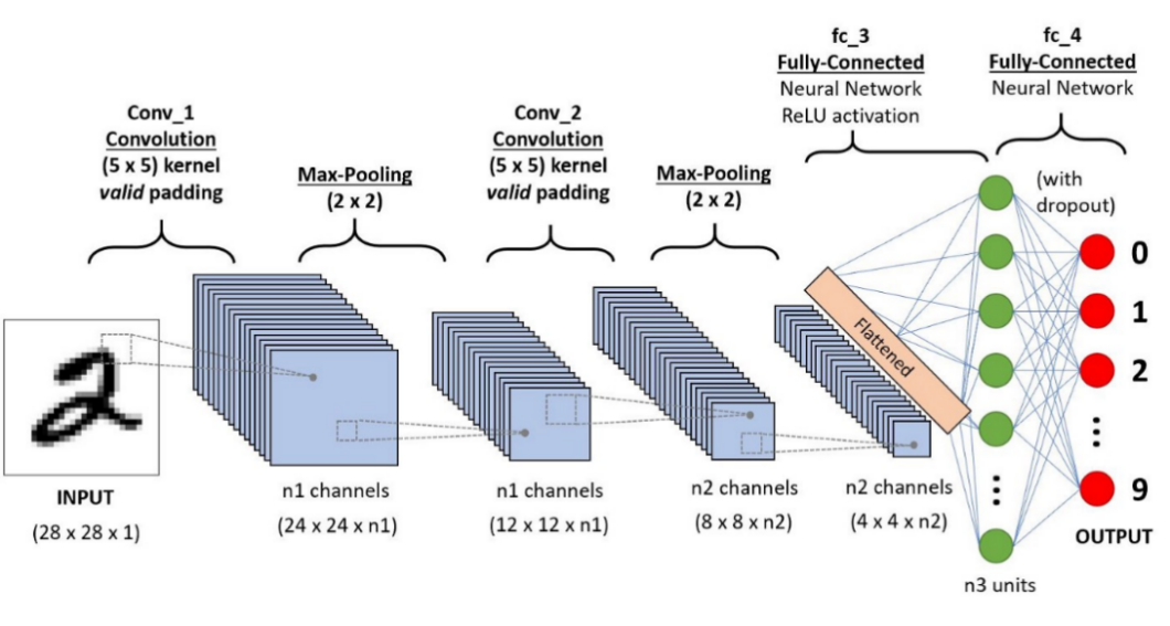
In a multiple layer neural network, each neuron will need to handle one input, so if the input is very big, for example, a picture of m times n pixels, and each pixel has a RGB value, that will make the input to be a three-dimensional data and will enormously increase the need for the number of neurons and their connection. However, CNN can reduce the problem and finally extract it into several essential features. To achieve this object, CNN has three layers: convolutional layer, pooling layer, and fully connected(FC) layer [14]. In the convolutional layer, a filter is moving over the input data, and creating a feature map for the pooling layer. The filter, or a kernel, a feature detector, is a two-dimensional array or a matrix, depending on the input data type. It will do a dot product with the input data, and the result is said to be the feature of this area and sent to the feature map, which is also an array or a matrix. Then the filter will move by a stride so that it will scan all areas on the input, and a completed feature map parsed to the next layer, pooling layer. The pooling layer also has a filter, but it does not have weights like that in the convolutional layer. It also sweeps the entire input and uses an aggregation function to downsize the dimension of the input. Then it comes down to the fully connected layer. As figure 9 shows, there could be multiple layers of convolution and pooling, so the fully connected layer will have limited nodes of neural network. Finally, the input data is transformed into low-level patterns and can be easily recognized by the neural network and passed to the output layer of the entire network [15].

6. Conclusion

Through the study of machine learning, it is now possible for computers to acquire knowledge without having it hard-coded into them. It can be supervised or unsupervised or semi-supervised. There are also reinforcement learning and neural networks. It is an ideal solution for tasks for computer vision and data science. The essence of the machine learning algorithm is to transform real life problem into mathematical problem, and utilize the computer’s power to solve it, and give the result back to real life. Machine learning is now being used in all walks of life and the algorithms behind it is what makes them productive. This paper made an introduction to all sub field of machine learning and their algorithms. However, there are still limitations for this paper because it does not dig into the mathematical essence of them. To improve this, further research can be done by establishing and reconstructing the algorithms and testing the mathematical formulas.

Acknowledgement

I want to show my appreciation to my professor who taught me academic writing in Kean University, who provided me with important guidance. Further, I want to thank my professors who helped me with learning all the knowledge about data science and machine learning. I also want to show my gratitude to my friends and family. Without their support, I wouldn’t have achieved what I have now.

References

[1]. P. P. Sarangi, M. Panda, S. Mishra, B. S. P. Mishra, and B. Majhi, Eds., 2022. Machine Learning for Biometrics. Academic Press.
[2]. V. Kotu and B. Deshpande, 2019. Data Science: Concepts and Practice. Cambridge: Morgan Kaufmann is an imprint of Elsevier.
[3]. G. Shobha and S. Rangaswamy, 2018. “Machine learning,” Handbook of Statistics, vol. 38, pp. 197–228.
[4]. S. Jaiswal, 2022, “Supervised machine learning—javatpoint,” www.javatpoint.com. [Online]. Available: https://www.javatpoint.com/supervised-machine-learning.
[5]. Y.-Y. Song and Y. Lu, 25-Apr-2015. “Decision tree methods: Applications for classification and prediction,” Shanghai archives of psychiatry, [Online]. Available: https://www.ncbi.nlm.nih.gov/pmc/articles/PMC4466856/.
[6]. “Overview of use of decision tree algorithms in machine learning,” IEEE Xplore, 27-Jun-2011. [Online]. Available: https://ieeexplore.ieee.org/abstract/document/5991826.
[7]. L. E. Peterson, 2022, “K-Nearest Neighbor,” Scholarpedia. [Online]. Available: http://scholarpedia.org/article/K-nearest_neighbor.
[8]. Z. Ghahramani, 2004. “Unsupervised learning,” Advanced Lectures on Machine Learning, pp. 72–112.
[9]. Szepesvári Csaba, 2010. Algorithms for reinforcement learning. Sand Rafael, CA: Morgan & Claypool.
[10]. “Monte Carlo method,” 2022, Monte Carlo Method — an overview|ScienceDirect Topics. [Online]. Available: https://www.sciencedirect.com/topics/medicine-and-dentistry/monte-carlo-method.
[11]. J.-S. Wang, Oct. 1999. “Transition matrix monte Carlo method,” Computer Physics Communications, vol. 121-122, pp. 22–25.
[12]. M. A. Nielsen, 2015. Neural networks and deep learning. Estats Units d'Amèrica: Determination Press.
[13]. S. Saha, “A comprehensive guide to Convolutional Neural Networks - the eli5 way,” A comprehensive guide to Convolutional Neural Network, 17-Dec-2018. [Online]. Available: https://towardsdatascience.com/a-comprehensive-guide-to-convolutional-neural-networks-the-eli5-way-3bd2b1164a53.
[14]. IBM Cloud Education, “What are convolutional neural networks?,” What are Convolutional Neural Networks?, 20-Oct-2020. [Online]. Available: https://www.ibm.com/cloud/learn/convolutional-neural-networks.
[15]. “Ann vs CNN vs RNN: Types of neural networks,” CNN vs. RNN vs. ANN – Analyzing 3 Types of Neural Networks in Deep Learning, 19-Oct-2020. [Online]. Available: https://www.analyticsvidhya.com/blog/2020/02/cnn-vs-rnn-vs-mlp-analyzing-3-types-of-neural-networks-in-deep-learning/.
Cite this article
Ling,Q. (2023). Machine learning algorithms review. Applied and Computational Engineering,4,91-98.
Data availability
The datasets used and/or analyzed during the current study will be available from the authors upon reasonable request.
Disclaimer/Publisher's Note
The statements, opinions and data contained in all publications are solely those of the individual author(s) and contributor(s) and not of EWA Publishing and/or the editor(s). EWA Publishing and/or the editor(s) disclaim responsibility for any injury to people or property resulting from any ideas, methods, instructions or products referred to in the content.
About volume
Volume title: Proceedings of the 3rd International Conference on Signal Processing and Machine Learning
© 2024 by the author(s). Licensee EWA Publishing, Oxford, UK. This article is an open access article distributed under the terms and
conditions of the Creative Commons Attribution (CC BY) license. Authors who
publish this series agree to the following terms:
1. Authors retain copyright and grant the series right of first publication with the work simultaneously licensed under a Creative Commons
Attribution License that allows others to share the work with an acknowledgment of the work's authorship and initial publication in this
series.
2. Authors are able to enter into separate, additional contractual arrangements for the non-exclusive distribution of the series's published
version of the work (e.g., post it to an institutional repository or publish it in a book), with an acknowledgment of its initial
publication in this series.
3. Authors are permitted and encouraged to post their work online (e.g., in institutional repositories or on their website) prior to and
during the submission process, as it can lead to productive exchanges, as well as earlier and greater citation of published work (See
Open access policy for details).