1. Introduction

Real estate developers and property investors benefit from knowing the trends of housing prices [1]. Furthermore, house price prediction can help potential buyers and sellers of homes manage their finances. The different features of a particular house, such as lot size and number of bedrooms, affect the price of the house. With house prices changing frequently in the real estate market, there has been an increasing need to accurately predict the prices of residential homes.

Machine learning models are important for house price prediction because they can efficiently consider the various features of a house and give an accurate estimate for its price using historical data. Different machine learning models provide different estimates for housing prices, and within each machine learning model, any hyperparameters can affect the estimate as well. Therefore, experiments were conducted to analyse different machine learning models with different hyperparameters for the task of house price prediction [2].

2. Methodology

In this section, we introduce several algorithms used in this paper.

2.1. Regression Tree

One of the most basic machine learning models is the regression tree [3], or a decision tree where the variables are continuous. The predictor space is defined as the set of values the features \( {A_{1}},{A_{2}},…,{A_{m}} \) can take on. The predictor space is divided up into \( G \) distinct and non-overlapping regions labeled \( {R_{1}},{R_{2}},…,{R_{G}} \) . The tree model makes the same prediction for every tuple \( x=({x_{1}},{x_{2}},…,{x_{m}}) \) in the same region \( {R_{g}} \) , namely, the mean value for that region.

A top-down, greedy algorithm called recursive binary splitting is used to construct the regions \( {R_{1}},{R_{2}},…,{R_{G}} \) . Starting from the top of the tree, at each node, the tree splits into two branches, corresponding to the current region \( {S_{k}} \) (subset of predictor space) splitting into two smaller regions. More specifically, a predictor \( {A_{j}} \) and cutoff \( s \) are chosen, and the two regions are \( \lbrace x{∈S_{k}}|{x_{j}} \lt s\rbrace \) and \( \lbrace x{∈S_{k}}|{x_{j}}≥s\rbrace \) . At the node corresponding to the region \( {S_{k}} \) , the optimal choices for the predictor \( {A_{j}}∈\lbrace {A_{1}},{A_{2}},…,{A_{m}}\rbrace \) and cutoff \( s∈R \) are such that the following quantity is minimized:

\( \sum _{i: {x_{i}}∈\lbrace x{∈S_{k}}|{x_{j}} \lt s\rbrace }{({y_{i}}-{\hat{y}_{1}})^{2}}+\sum _{i: {x_{i}}∈\lbrace x{∈S_{k}}|{x_{j}}≥s\rbrace . }{({y_{i}}-{\hat{y}_{2}})^{2}}\ \ \ (1) \)

where \( {x_{i}} \) = values of features of \( i \) th data point in respective set, \( {y_{i}} \) = value of target variable associated with \( {x_{i}} \) , \( {\hat{y}_{1}} \) = mean value of \( {y_{i}} \) for \( \lbrace x{∈S_{k}}|{x_{j}} \lt s\rbrace \) , \( {\hat{y}_{2}} \) = mean value of \( {y_{i}} \) for \( \lbrace x{∈S_{k}}|{x_{j}}≥s\rbrace \) . The tree splitting process continues until a stopping criterion is reached.

2.2. Random Forest

Another supervised machine learning method is random forest [4]. This type of model combines multiple base models to produce a new model, so it is called an ensemble method. In a random forest model, \( B \) random (potentially overlapping) subsets of the training data are selected. For each subset, a regression tree is built using that data. The main difference between such a regression tree and the regression tree model in Section 2.1 is that in generating a particular regression tree in a random forest, for every possible tree split, only some of the possible predictor variables are allowed to be candidates for the predictor variable used in that split. Usually, there are \( d≈\sqrt[]{m} \) candidates, meaning that most of the \( m \) predictor variables are not considered for the split. Note that each split may have different candidates.

After all \( B \) regression trees are built, the final random forest model is generated by taking the average of the regression tree models:

\( {f_{avg}}(x)=\frac{1}{B}\sum _{b=1}^{B}{f_{b}}(x)\ \ \ (2) \)

where \( {f_{b}}(x) \) = target function for \( b \) th subset of training data.

A random forest model is usually more accurate than a single regression tree. A disadvantage of the single regression tree model is that it has high variance, meaning that if a different training set were used, the resulting model could be significantly different. Since averaging a set of independent observations \( {Z_{1}},{Z_{2}},…,{Z_{n}} \) reduces variance, a random forest model would have a lower variance error than a single regression tree.

Furthermore, allowing only \( d≈\sqrt[]{m} \) of the \( m \) predictor variables to be candidates at each tree split, instead of all \( m \) features, results in the tree model predictions being less similar, since the strongest predictor variables will no longer always be at the top split. Taking the average of uncorrelated predictions reduces variance more than taking the average of correlated predictions, which adds on to the effectiveness of the random forest model.

2.3. Gradient Boosting

Like random forest, gradient boosting is a supervised learning ensemble method [5]. Unlike in random forest, where the regression trees are all created independently of each other, in gradient boosting each new model attempts to correct the errors made by the previous model by minimizing a differentiable loss function. The iterative process of minimizing a loss function has the effect of improving the overall model over time, i.e. reducing the overall error. A common loss function is squared-error:

\( L(y,F)={(y-F)^{2}}\ \ \ (3) \)

The following is an algorithm for gradient boosting that runs for \( M \) iterations on a training set \( \lbrace {(x_{1,}}{y_{1}}),…{,(x_{n,}}{y_{n}})\rbrace \) . Steepest descent with negative gradient is used to minimize the differentiable loss function.

1) Initialize a constant function \( {F_{0}}(x) \) .

2) For \( m=1 \) to \( M \) :

Calculate \( -[\frac{∂L({y_{i}},F({x_{i}}))}{∂F({x_{i}})}] \) for \( i=1 \) to \( n \) .

Fit a regression tree model \( {h_{m}}(x) \) to the negative gradients.

Update the new model to be

\( {F_{m}}(x)={F_{m-1}}(x)+{λ_{m}}{h_{m}}(x) \)

for some constant \( {λ_{m}} \) .

3) The resulting model is \( {F_{M}}(x) \) .

2.4. XGBoost

XGBoost is a popular boosting algorithm that many data scientists have used to win machine learning competitions [6]. XGBoost is highly optimized, as it can handle sparse data easily and use weighted quantiles to determine where to split. XGBoost is also scalable, as it uses out-of-core computation as well as parallel and distributed computing to handle large data with relatively few cluster resources.

For tree learning, or more specifically, finding the optimal split, there is an algorithm called exact greedy algorithm, which involves sorting the data based on feature values. Although this algorithm is accurate, there is not enough memory to include all the data in practice. Therefore, XGBoost uses an approximate algorithm. This algorithm finds the optimal split by aggregating various statistics. The algorithm has two versions: global proposal and local proposal. In global proposal, the candidate splits are proposed when the tree is constructed in the beginning, and the proposals are kept constant for all levels. Meanwhile, in local proposal, the proposals may be changed after every split. Although the local version has more proposal steps, it is more effective for deeper trees.

2.5. LightGBM

LightGBM is a boosting algorithm with histogram-based algorithms [7]. One significant benefit of LightGBM is that it trains models faster and consumes less memory than other machine learning models.

The algorithms used in LightGBM are optimized for different tasks. The feature parallel algorithm in LightGBM helps parallelize the task of finding the best split in the decision tree. The data parallel algorithm helps parallelize the whole decision learning process. Since high-dimensional data tends to be sparse, LightGBM bundles exclusive features into much fewer dense features, a technique called Exclusive Feature Bundling (EFB). LightGBM also uses gradient-based one-side sampling, which reduces the amount of data used while also maintaining decision tree accuracy. Overall, LightGBM is an efficient machine learning technique.

3. Experiments

3.1. Datasets

The dataset used in this study describes residential homes sold in Ames, Iowa in the United States from 2006 to 2010 [8]. The dataset has a size of 1460 rows and 81 columns. In each row of the dataset, 79 variables are used to describe aspects of a particular residential home, and the SalePrice variable is used to store the price of that home.

3.2. Experimental Settings

Machine learning models often have hyperparameters, which are parameters that can be set to control the learning process. In the experiments, various hyperparameters for the single regression tree, random forest, and XGBoost models were analysed to see which values made each model perform the best. For each of these experiments, identical models were created, with the only difference between them being different values of a single hyperparameter. Then, the error (Section 3.3) for each model was recorded.

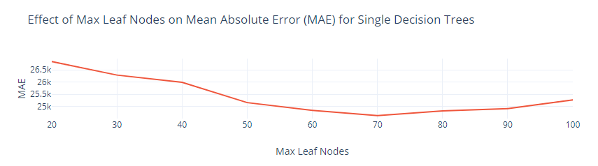
One hyperparameter for the single regression tree is the maximum number of leaf nodes. A tree with too few leaf nodes can underfit the data, while a tree with too many leaf nodes can overfit the data. To find the optimal value for the maximum number of leaf nodes for a single regression tree, the values of the hypermeter tested were 20, 30, 40, … 100, i.e. a constant difference of 10 from 20 to 100.

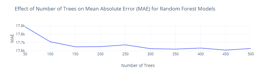
The number of weak learners is a hyperparameter for the random forest model. The weak learners are usually regression trees, which are used in the averaging step of the algorithm. Having more weak learners tends to make the model more accurate in making predictions [9]. In the experiments, the values of the hyperparameter tested were 50, 100, 150, … 500, i.e. a constant difference of 50 from 50 to 500.

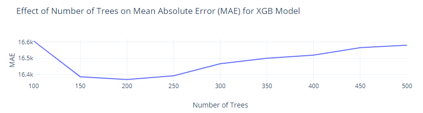
The XGBoost model has the number of weak learners as a hyperparameter. Having more weak learners and a small learning rate tends to make the model’s predictions more accurate. In the experiments, the values of the hyperparameter tested were 100, 150, 200, … 500, i.e. a constant difference of 50 from 100 to 500 [10]. The computational machine used for running the experiments had a 7th Gen Intel® Core™ i7-7500 CPU with a base frequency of 2.70 GHz, as well as 8.00 GB of installed RAM.

3.3. Metrics

The metric used in the experiments is the mean absolute error (MAE):

\( MAE=\frac{\sum _{i=1}^{n}|{y_{i}}-y_{i}^{*}|}{n}\ \ \ (4) \)

where \( n \) = total number of data points, \( {y_{i}} \) = actual value in \( i \) th data point, \( y_{i}^{*} \) = predicted value in \( i \) th data point. A lower mean absolute error signifies better predictive accuracy.

3.4. Pre-processing

Missing values can be handled by dropping columns with missing values or imputing them. In imputation, each missing value (NaN) in a column with numerical data is replaced with a number, such the mean of the non-missing values in the column.

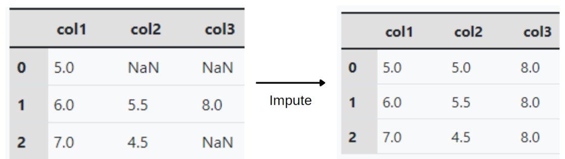
In the experiments, two random forest models were set up with the two models being identical, except one model had the columns with missing values dropped, while the other model used imputing for the missing values. Then, the mean absolute errors of the two random forest models were recorded and compared to determine the effectiveness of each approach.

Meanwhile, categorical data can be handled by dropping columns with categorical data or using one-hot encoding. The latter is a process in which new binary columns are created, with each column recording whether each training example in the original data had a certain value for a particular feature.

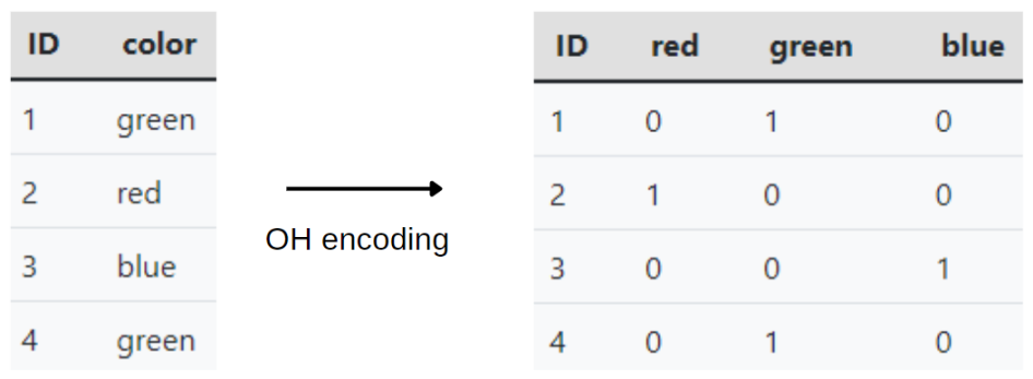
In the experiments, two identical random forest models were set up, with the only difference being how each handled categorical data. The mean absolute errors of the two random forest models were then recorded and compared to determine the effectiveness of each approach.

3.5. Results and Analysis

In the experiments, missing values were best handled by imputation. The model that used imputation had an MAE of 17809, while the model that dropped columns with missing values had an MAE of 18852. Meanwhile, the optimal way to handle columns with categorical data was one-hot encoding. The model that used a one-hot encoder had an MAE of 17628, while the model that dropped columns with categorical data had an MAE of 17977.

For the single regression tree, having a maximum of 70 leaf nodes was optimal, with the result being an MAE of 24632. For random forest, having 450 regression trees was optimal, with the result being an MAE of 17609. For XGBoost, having 200 trees was optimal, with the result being an MAE of 16370.

Table 1. Handling missing values.

Table 2. Handling categorical data.

The machine learning model with the lowest MAE in the dataset was XGBoost. The machine learning models with slightly higher MAEs were gradient boosting and LightGBM. The random forest model had a higher MAE, and the single regression tree model had the highest MAE.

4. Conclusion

As seen in the experiments for house price prediction, the optimal way to handle missing values is to impute them, and the optimal way to handle categorical columns is to use one-hot encoding. Other methods, such as removing columns with missing values or categorical columns, may produce less accurate models. Furthermore, many machine learning models, including XGBoost and random forest, have modifiable parameters that can be optimized to produce accurate models. The most accurate machine learning models are XGBoost, gradient boosting, and LightGBM, as seen in the house price prediction experiments. Possible future work includes analyzing more hyperparameters (e.g. the learning rate for XGBoost) and applying machine learning models to other real-world scenarios.

References

[1]. Cerda, P., Varoquaux, G., & Kégl, B. (2018). Similarity encoding for learning with dirty categorical variables. Machine Learning, 107(8), 1477–1494. doi:10.1007/s10994-018-5724-2.
[2]. Chen, T., & Guestrin, C. (2016). XGBoost: A Scalable Tree Boosting System. Proceedings of the 22nd ACM SIGKDD International Conference on Knowledge Discovery and Data Mining, 785–794. San Francisco, California, USA. doi:10.1145/2939672.2939785
[3]. Cock, D. D. (2011). Ames, Iowa: Alternative to the Boston Housing Data as an End of Semester Regression Project. Journal of Statistics Education, 19(3), null. doi:10.1080/10691898.2011.11889627
[4]. Cort J. Willmott, & Kenji Matsuura. (2005). Advantages of the mean absolute error (MAE) over the root mean square error (RMSE) in assessing average model performance. Climate Research, 30(1), 79–82. doi:10.3354/cr030079
[5]. Donders, A. R. T., van der Heijden, G. J. M. G., Stijnen, T., & Moons, K. G. M. (2006). Review: A gentle introduction to imputation of missing values. Journal of Clinical Epidemiology, 59(10), 1087–1091. doi:10.1016/j.jclinepi.2006.01.014
[6]. Friedman, J. H. (2001). Greedy function approximation: A gradient boosting machine. The Annals of Statistics, 29(5), 1189–1232. doi:10.1214/aos/1013203451
[7]. Hastie, T., Friedman, J., & Tisbshirani, R. (2017). The Elements of Statistical Learning: Data Mining, Inference, and Prediction. Springer.
[8]. James, G., Witten, D., Hastie, T., & Tibshirani, R. (2021). An Introduction to Statistical Learning: with Applications in R. Springer.
[9]. Ke, G., Meng, Q., Finley, T., Wang, T., Chen, W., Ma, W., … Liu, T.-Y. (2017). LightGBM: A Highly Efficient Gradient Boosting Decision Tree. Proceedings of the 31st International Conference on Neural Information Processing Systems, 3149–3157. Long Beach, California, USA. Red Hook, NY, USA: Curran Associates Inc.
[10]. Zulkifley, N., Rahman, S., Nor Hasbiah, U., & Ibrahim, I. (12 2020). House Price Prediction using a Machine Learning Model: A Survey of Literature. International Journal of Modern Education and Computer Science, 12, 46–54. doi:10.5815/ijmecs.2020.06.04.
Cite this article
Fang,L. (2023). Machine learning models for house price prediction. Applied and Computational Engineering,4,409-415.
Data availability
The datasets used and/or analyzed during the current study will be available from the authors upon reasonable request.
Disclaimer/Publisher's Note
The statements, opinions and data contained in all publications are solely those of the individual author(s) and contributor(s) and not of EWA Publishing and/or the editor(s). EWA Publishing and/or the editor(s) disclaim responsibility for any injury to people or property resulting from any ideas, methods, instructions or products referred to in the content.
About volume
Volume title: Proceedings of the 3rd International Conference on Signal Processing and Machine Learning
© 2024 by the author(s). Licensee EWA Publishing, Oxford, UK. This article is an open access article distributed under the terms and
conditions of the Creative Commons Attribution (CC BY) license. Authors who
publish this series agree to the following terms:
1. Authors retain copyright and grant the series right of first publication with the work simultaneously licensed under a Creative Commons
Attribution License that allows others to share the work with an acknowledgment of the work's authorship and initial publication in this
series.
2. Authors are able to enter into separate, additional contractual arrangements for the non-exclusive distribution of the series's published
version of the work (e.g., post it to an institutional repository or publish it in a book), with an acknowledgment of its initial
publication in this series.
3. Authors are permitted and encouraged to post their work online (e.g., in institutional repositories or on their website) prior to and
during the submission process, as it can lead to productive exchanges, as well as earlier and greater citation of published work (See
Open access policy for details).