1. Introduction

Load forecasting is regarded as a fundamental element in ensuring the secure and stable operation of power systems and optimizing resource allocation for the operation and dispatch of modern power systems. Particularly in the context of high penetration of renewables and the intricate interaction of diverse loads, precise forecasting serves as a critical enabler for addressing uncertainties and enhancing grid resilience and economic efficiency [1-2]. According to the length of the forecasting horizon, the power load forecasting problem is generally categorized into long-term and short-term predictions. Short-term load forecasting, ranging from hourly to weekly scales, is considered a critical component of various stages in power grid operation, which impacts the efficient implementation of system arranging and production methodologies [3]. Ultra-short-term load forecasting, which is used for online monitoring of power equipment's operational status, typically provides load variations for the next few minutes to several hours. With the advancement of market-oriented reforms, the balance between electricity supply and demand is increasingly dependent on real-time trading mechanisms, making the accuracy of short-term load forecasting critically important. High-accuracy load forecasting not only reduces grid operation costs and improves economic efficiency but also effectively responds to potential load variations and unforeseen events, guaranteeing the safe and reliable operation of the entire system [4]. The expansion of smart grid infrastructure and digital upgrades significantly enhance the data collection frequency and accuracy in dispatching systems, which in turn provides a massive and high-quality data base for analyzing load characteristics and implementing deep learning methods.

Conventional load forecasting primarily relies on statistical analytic techniques, such as time series analysis [5], multiple linear regression [6], and exponential smoothing [7]. These strategies are based on the correlation between energy consumption and factors such as historical usage and external conditions, and regression models are fitted to the data to forecast future load. However, considering the advancement of contemporary power systems, the integration of diverse loads, high proportions of renewable energy, and the inherent randomness of renewables have made load variations increasingly complex and highly nonlinear, rendering traditional forecasting methods unable to achieve satisfactory performance [8]. The emergence of next-generation artificial intelligence technologies has facilitated the extensive use of data-driven artificial intelligence approaches in load forecasting for power systems. Data analysis techniques based on conventional machine learning and deep learning, with their strong ability to extract complex abstract features, have exhibited superior accuracy in anticipating outcomes within the domain of load prediction. In contemporary research, the utilization of artificial intelligence in power load prediction is extensively explored by numerous scholars. Literature [9] proposes a statistical method based on annual cycle pattern decomposition, which significantly improves the forecasting accuracy of the autoregressive integrated moving average (ARIMA) model and the Exponential Smoothing State Space (ETS) model by encoding monthly electricity demand series into standardized patterns. Literature [10] proposes a hybrid statistical framework based on the Generalized Additive Model (GAM) and the Seasonal Autoregressive Integrated Moving Average (SARIMA) model. By integrating exogenous variables with time series characteristics, it effectively captures the seasonality and annual growth rate of load, demonstrating excellent performance in long-term forecasting. Literature [11] employs a hybrid model framework combining the Prophet time series model with Bayesian optimization (BO) and the eXtreme Gradient Boosting (XGBoost) model, significantly reducing the overfitting risk inside intricate nonlinear environments. Literature [12] constructs a hybrid model combining Convolutional Neural Network (CNN), Long Short-Term Memory (LSTM), and Transformer-Gaussian Process (GP) through a multivariate data fusion strategy, substantially enhancing the precision of power load forecasting. Literature [13] develops a Temporal Convolutional Network (TCN) model optimized by the Improved Salp Swarm Algorithm (ISSA) to meet the complexity and high-precision demands of short-term urban power load forecasting. The integration of the Error Auxiliary Model (EAM) within the ISSA-TCN+EAM prediction framework improves the model's capacity to identify the nonlinear characteristics of power load, while error correction strategies are employed to further improve forecasting stability. However, certain limitations are still encountered in existing research. Many approaches tend to suffer from overfitting or underfitting when handling data diversity. Meanwhile, high computational complexity and intensive resource requirements restrict their practical application in power grid scheduling, potentially reducing operational efficiency.

Literature [14] designs a hybrid model that integrates CNN, LSTM, and a multi-modal attention mechanism, enhancing global feature modeling through a multi-head self-attention mechanism. Literature [15] proposes a short-term forecasting model that combines principal component analysis with LSTM neural networks, and verifies that the model can capture the dynamic characteristics of time series data. However, the precision and reliability of LSTM forecasting models are highly dependent on preset parameters. Most of the existing LSTM models rely on empirically determined parameters, resulting in limited generalization ability and insufficient prediction accuracy and stability. Improper optimization can not only impact the overall performance of the model but also increase the training time of the network.

The quantum-behaved particle swarm optimization (QPSO) algorithm is employed to enhance the LSTM network, aiming to address the insufficient predictive precision and stability of individual LSTM models. A QPSO-LSTM forecasting model is constructed and applied to ultra-short-term power load prediction. Through the integration of quantum behavior modeling, probability distribution mechanisms, and dynamic parameter adjustment, the QPSO algorithm enhances both global and local search capabilities, thereby significantly improving predictive precision and reliability of the model. Initially, the power load data is normalized through preprocessing. Subsequently, the key hyperparameters of LSTM are globally optimized by QPSO to construct the QPSO-LSTM forecasting model. Finally, the predictive efficacy of the LSTM, PSO-LSTM, and QPSO-LSTM models is compared and validated through case studies, demonstrating the efficacy of QPSO optimization in enhancing the forecasting precision and fitting capability of LSTM.

2. Prediction model based on QPSO-LSTM

2.1. LSTM neural network

LSTM is a specialized type of Recurrent Neural Network (RNN) designed for the analysis of sequential and time series data, specifically to mitigate the vanishing and exploding gradient issues prevalent in conventional RNNs. LSTM analyzes the temporal features of data through three key gating units: the forget gate, the input gate, and the output gate [16-17]. The basic unit of the network is shown in Figure 1. In the hidden layer, a memory unit is added in LSTM, consisting of a "cell state" vector, represented as . is employed to store historical information and transfer the current state information to the next time step, granting the model long-term memory ability, which shows good performance in processing long time-series data.

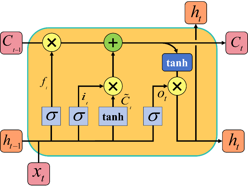
Figure 1: Basic unit of LSTM network

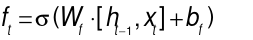
The mathematical expressions corresponding to the internal structure of the LSTM unit are shown in equations (1) to (6):

(1)

(2)

(3)

(4)

(5)

(6)

The forget gate regulates the degree to which historical information in the cell state is eliminated. In equation (1), denotes the output of the forget gate at time t. The previous hidden state and the current input vector are fed into the sigmoid activation function ; a value of close to 0 indicates that the corresponding information is forgotten, while a value close to 1 means it is retained.

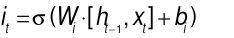
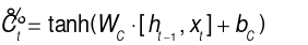
The input vector in the input gate is transformed by both the sigmoid and tanh functions, and these transformations together decide the retained vector in the state memory unit. In equation (2), represents the output of the input gate after being processed by the sigmoid function. In equation (3), the candidate cell state is the output of the input gate after being processed by the tanh function. multiplies with to decide which information is discarded or preserved.

The output of the forget gate is multiplied by the previous cell state, and then the product of the input gate and the candidate cell state is added to obtain the new cell state. The state update rule is shown in equation (4). In equation (5), denotes the output of the output gate. In equation (6), is the current hidden state, which serves as the input for the next time step.

represents the bias terms corresponding to different gate units. represents the weight matrices associated with different gate units.

2.2. QPSO algorithm

Particle Swarm Optimization (PSO) is an optimization algorithm that emulates the motion of particles in the search space, achieving global optimization through the sharing of individual experience and group information. The current state of each particle is determined by its previous state, its own best state, and the group’s best state. Particles update their states through individual optimization and group evolution, continuously learning to improve their states [18]. The particle update equation is presented as follows:

(7)

(8)

denotes the velocity vector of the i-th particle at the k-th iteration; represents the position vector of the i-th particle at the same iteration; is the historical best position of the i-th particle; and is the global best position among all particles. denotes the inertia weight, which controls the influence of the particle’s previous velocity. are the acceleration coefficient, and are uniformly distributed random numbers in the range [0,1] at the k-th iteration, used to introduce randomness and augment the stochastic algorithmic search capabilities. Equation (8) updates the particle's position using the velocity vector , yielding a new position at the (k+1)-th iteration.

Nevertheless, the absence of random positional changes often results in a lack of diversity among particles, making the algorithm susceptible to local optima in high-dimensional search spaces. Specifically, the performance of PSO is highly determined by key parameters like and .An excessively large may lead to over-exploration, while a small value may result in insufficient exploitation, making parameter tuning challenging. At later iterations, the particles converge toward , resulting in a substantial decrease in swarm diversity. There is no effective diversity-preserving mechanism within the velocity update formula.

QPSO utilizes quantum states to represent particle motion, and optimization is conducted by emulating particle dynamics in quantum space. In quantum space, the position update of each particle no longer uses the classic velocity and position update formulas but instead uses a quantum transition probability distribution to update the particle’s position. This method exhibits greater randomness, which effectively overcomes the limitations of conventional PSO. Particles are allowed to appear in regions far from the current optimum with a certain probability, thereby maintaining population diversity. Moreover, the dependency on parameters is minimized in QPSO, as the search scope is adaptively regulated through the quantum potential well mechanism.

The optimization steps of QPSO are described by the expressions in Equations (9) to (11):

(9)

Equation (9) defines the mean best position of all particles as . represents the swarm size, and denotes the individual optimal location of the i-th particle at the k-th iteration.

(10)

Equation (10) defines the position update equation for the particles. Where a value equally distributed within the interval (0, 1), and represents the global optimal location of the i-th particle during the k-th iteration.

(11)

Equation (11) defines the iterative equation for particle movement. Where represents a randomly changing number in the range (0, 1), used to determine the direction of the particle’s position update. represents the contraction-expansion coefficient, which affects the algorithm's convergence rate. When > 1, the particle searches globally; when < 1, it converges toward .

2.3. QPSO-LSTM prediction algorithm

The performance of LSTM in load forecasting is highly dependent on the configuration of hyperparameters, including the quantity of hidden layer nodes, learning rate, and number of iterations. Conventional empirical parameter adjustment is inefficient and tends to result in convergence to local optima. Therefore, a hyperparameter optimization strategy based on QPSO is employed to optimize the key parameters of the LSTM model. In comparison with PSO, the quantum-inspired position updating mechanism of QPSO improves population diversity and eliminates dependence on historical velocity during particle position updates. The algorithm structure is simplified by the use of a single control parameter, the contraction-expansion coefficient .

In this paper, QPSO is used to optimize four key parameters of LSTM—the number of hidden layer nodes, the number of training iterations, and the learning rate. The quantity of hidden layer nodes is set within the integer range of 1 to 200. The number of training iterations is defined within the range of 10 to 100, and the learning rate is treated as a floating-point parameter between 0.001 and 0.01. The optimization process uses an iterative search strategy to efficiently explore the parameter space. The specific steps for modeling the QPSO-LSTM prediction model are as follows:

1.Data preprocessing: To eliminate the influence of feature scale differences on the optimization process, the power load data is normalized and then divided into training and testing sets.

2.Initialize particle swarm: Each particle in the swarm is used to represent a potential set of parameters for the LSTM network, including swarm size, particle dimension, iteration count, and particle position. These parameters are randomly initialized within the predefined search space.

3.Evaluate fitness: the particle location data serve as parameters for training the LSTM model, while the Mean Squared Error (MSE) is utilized as the fitness function to evaluate each particle's fitness.

4.Update particle position: Based on the fitness values, the optimal solution for each particle’s individual and the global best solution for the swarm are identified, and the particle positions are updated accordingly. The updated particle positions (i.e., new parameter combinations) are re-evaluated, and their fitness values are updated accordingly.

5.Steps c and d are repeated until the best particle position is found or the QPSO algorithm reaches the maximum iteration limit, at which point the QPSO optimization process is terminated.

6.The optimal global value is provided to the LSTM network for hyperparameter optimization. The model is subsequently employed to forecast the sample data from the test set.

3. Analysis of examples

3.1. Data preprocessing and parameter setting

In this paper, electricity load data from a certain region are used as the dataset, with data updated every 15 minutes. The data is partitioned into training and test sets sequentially, allocating 70% for training and 30% for testing. Time series samples are generated with the sliding window method, wherein data from the preceding 10 time steps serve as inputs to forecast the following 2 time steps. The max-min normalization method in Equation (12) is applied to process the power load data, scaling the normalized data into the [0, 1] range to facilitate model training and optimization.

(12)

The particle swarm size M is established at 30. The iteration limit is established at 200 to guarantee complete convergence of the algorithm and prevent premature cessation. The particle dimension D is set to 4, corresponding to the four optimization parameters: the quantity of nodes in the two hidden layers, the number of training epochs, and the learning rate. This case study is implemented in the MATLAB R2022b programming environment. The Adam optimizer is used for training, with the mini-batch size set to 16.

3.2. Evaluation criteria

The model prediction accuracy evaluation metrics selected in this paper are the root mean square error (RMSE), mean absolute error (MAE), mean absolute percentage error (MAPE), and the coefficient of determination . Each metric quantifies the deviation between the predicted values and the actual values from different perspectives. The specific expressions are presented in Equations (13) to (16).

(13)

(14)

(15)

(16)

The RMSE amplifies larger errors and reflects the overall dispersion of the forecast results. The MAE reflects the average deviation between the predicted and actual values. The MAPE expresses the relative size of the prediction error in percentage terms and is used for comparative analysis of different methods. The smaller the values of these three indicators, the higher the prediction accuracy, the smaller the relative error, and the more effective the fitting of the model. measures the model's fit to the load data, with a value closer to 1 indicating stronger ability to capture data characteristics, and it is suitable for comparing the fitting performance of different models.

3.3. Experimental results analysis

The QPSO-LSTM model, PSO-optimized LSTM model, and LSTM model are constructed with the training set data for load forecasting, and the prediction outcomes are compared based on evaluation metrics. The comparison of prediction evaluation metrics is shown in Table 1.

Table 1: Comparison of prediction performance for different models

The prediction accuracy of the model has shown a significant enhancement when compared to the conventional LSTM model after optimization with PSO and QPSO. Among them, the PSO-LSTM and QPSO-LSTM models outperform the LSTM model in terms of RMSE, MAE, and MAPE metrics. The QPSO-LSTM model achieves the smallest values in all three metrics, further demonstrating the efficacy of the QPSO algorithm in improving model prediction stability and accuracy. The QPSO-LSTM model possesses the highest , indicating that it provides the best fit for the load data.

To provide a more intuitive comparison between different models, the prediction results are generated and compared, as shown in Figure 2. The LSTM curve exhibits a notable deviation from the actual values, especially in areas with large load fluctuations, where it fails to effectively capture the load variation trend. Compared to LSTM, the PSO-LSTM curve is closer to the real values and responds better to load fluctuations, but there are still delays or amplitude deviations in some areas. The prediction accuracy and fitting performance of the QPSO-optimized LSTM model are generally comparable to those of the PSO-LSTM model, but slightly better at peak points. The QPSO-LSTM curve fits the real values the best. This performance is consistent with the conclusions drawn from metrics such as RMSE, MAE, and MAPE, further validating the improvement in model performance brought by the optimization algorithm, with QPSO showing the most significant effect. The method effectively addresses the randomness of manual hyperparameter tuning in LSTM by leveraging the global search capability of QPSO, providing a viable solution for parameter optimization in power load forecasting models.

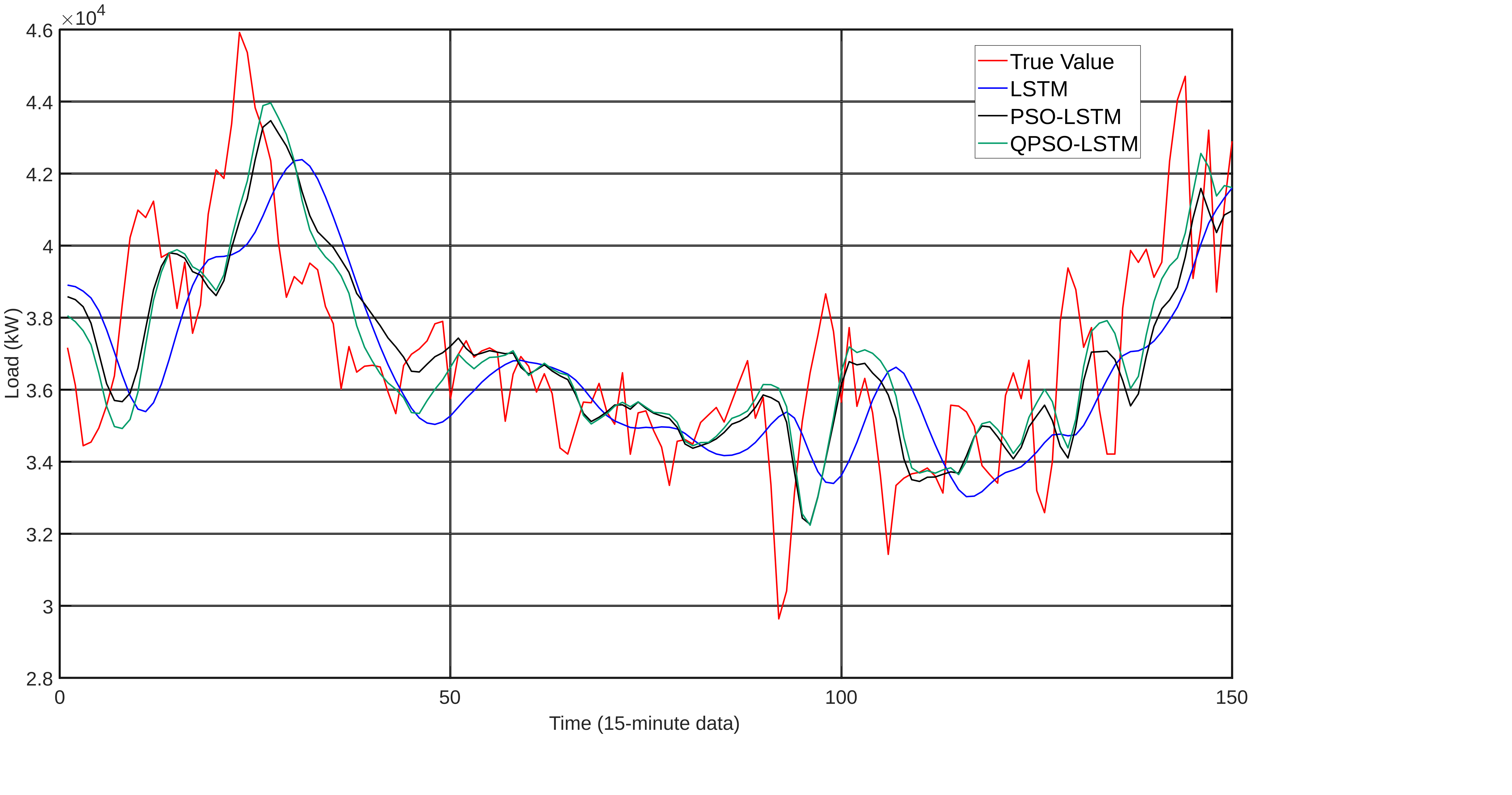
Figure 2: Comparison of prediction results of various models

4. Conclusion

This paper introduces a novel approach integrating quantum-behaved particle swarm optimization (QPSO) with long short-term memory (LSTM) networks to enhance ultra-short-term power load forecasting. By leveraging QPSO’s global search capability, critical LSTM parameters—including hidden layer node count, learning rate, and training iterations—are systematically optimized, addressing the limitations of manual empirical tuning in conventional LSTM frameworks. The methodology begins with normalizing raw load data and partitioning it into training and testing subsets. Subsequently, the QPSO-driven swarm iteratively explores parameter combinations to refine the LSTM architecture. Validated through empirical case studies, the optimized QPSO-LSTM model demonstrates superior performance compared to LSTM and PSO-LSTM variants. Quantitative evaluation using RMSE, MAE, and MAPE metrics reveals significant accuracy improvements, while the highest value confirms enhanced data-fitting capability. This method achieves a synergistic optimization of prediction accuracy and fitting capability under high fluctuation load scenarios, providing an efficient and reliable solution for load forecasting in power systems characterized by substantial renewable energy penetration.

References

[1]. Han, F.J., Wang, X.H., Qiao, J., et al. A review of artificial intelligence-based load forecasting in new power systems [J]. Proceedings of the CSEE, 2023, 43(22): 8569-8592. DOI:10.13334/j.0258-8013.pcsee.221560.
[2]. Habbak H, Mahmoud M, Metwally K, et al. Load forecasting techniques and their applications in smart grids[J]. Energies, 2023, 16(3): 1480.
[3]. Kondaiah, V.; Saravanan, B.; Sanjeevikumar, P.; Khan, B. A review on short-term load forecasting models for micro-grid application. J. Eng. 2022, 2022, 665– 689.
[4]. Ahmad, N.; Ghadi, Y.; Adnan, M.; Ali, M. Load forecasting techniques for power system: Research challenges and survey. *IEEE Access* 2022, 10, 71054–71090.
[5]. Paparoditis, E.; Sapatinas, T. Short-Term Load Forecasting: The Similar Shape Functional Time Series Predictor. IEEE Trans. Power Syst. 2013, 28, 3818– 3825.
[6]. Lei, S.; Sun, X.; Zhou, Q.; Zhang, X. Research on multivariate time series linear regression forecasting method for short-term load of electricity. Proc. CSEE 2006, 1, 27– 31.
[7]. Song, K.; Ha, S.; Park, J.W. Hybrid load forecasting method with analysis of temperature sensitivities. IEEE Trans. Power Syst. 2006, 21, 869– 876.
[8]. Alhamrouni, I.; Kahar, H.A.; Salem, M.; Swadi, M.; Zahroui, Y.; Kadhim, D.J.; Mohamed, F.A.; Nazari, M.A. A Comprehensive Review on the Role of Artificial Intelligence in Power System Stability, Control, and Protection: Insights and Future Directions. Appl. Sci. 2024, 14, 6214
[9]. PELKA P. Analysis and Forecasting of Monthly Electricity Demand Time Series Using Pattern-Based Statistical Methods[J/OL]. Energies, 2023, 16(2): 827. DOI:10.3390/en16020827.
[10]. ROYAL E, BANDYOPADHYAY S, NEWMAN A, et al. A statistical framework for district energy long-term electric load forecasting[J]. Applied Energy, 2025, 384: 125445.
[11]. ZENG S, LIU C, ZHANG H, et al. Short-term load forecasting in power systems based on the Prophet-BO-XGBoost model[J]. Energies, 2025, 18(2): 227.
[12]. ÖZEN S, YAZICI A, ATALAY V. Hybrid deep learning models with data fusion approach for electricity load forecasting[J]. Expert Systems, 2025, 42(2): e13741. DOI: 10.1111/exsy.13741.
[13]. Fan C, Li G, Xiao L, Yi L, Nie S. An ISSA-TCN short-term urban power load forecasting model with error factor[J]. Physica Scripta, 2025, 100: 045222.
[14]. GUO W, LIU S, WENG L, et al. Power Grid Load Forecasting Using a CNN-LSTM Network Based on a Multi-Modal Attention Mechanism[J]. Applied Sciences, 2025, 15: 2435. DOI:10.3390/app15052435.
[15]. Song Shaojian and Li Bohan, Short-term forecasting method of photovoltaic power based on LSTM. Renewable Energy Resources, 2021, 39(5): 594– 602.
[16]. Masood, Z.; Gantassi, R.; Choi, Y. Enhancing Short-Term Electric Load Forecasting for Households Using Quantile LSTM and Clustering-Based Probabilistic Approach. IEEE Access 2024, 12, 77257– 77268.
[17]. Liu, Y.; Liang, Z.; Li, X. Enhancing Short-Term Power Load Forecasting for Industrial and Commercial Buildings: A Hybrid Approach Using TimeGAN, CNN, and LSTM. IEEE Open J. Ind. Electron. Soc. 2023, 4, 451– 462.
[18]. Xie, T.; Zhang, Y.; Zhang, G.; Zhang, K.; Li, H.; He, X. Research on electric vehicle load forecasting considering regional special event characteristics. Front. Energy Res. 2024, 12, 1341246.
Cite this article
Tian,R. (2025). Artificial Intelligence-Based Ultra-Short-Term Power Load Forecasting. Applied and Computational Engineering,172,1-10.
Data availability
The datasets used and/or analyzed during the current study will be available from the authors upon reasonable request.
Disclaimer/Publisher's Note
The statements, opinions and data contained in all publications are solely those of the individual author(s) and contributor(s) and not of EWA Publishing and/or the editor(s). EWA Publishing and/or the editor(s) disclaim responsibility for any injury to people or property resulting from any ideas, methods, instructions or products referred to in the content.
About volume
Volume title: Proceedings of CONF-FMCE 2025 Symposium: Semantic Communication for Media Compression and Transmission
© 2024 by the author(s). Licensee EWA Publishing, Oxford, UK. This article is an open access article distributed under the terms and
conditions of the Creative Commons Attribution (CC BY) license. Authors who
publish this series agree to the following terms:
1. Authors retain copyright and grant the series right of first publication with the work simultaneously licensed under a Creative Commons
Attribution License that allows others to share the work with an acknowledgment of the work's authorship and initial publication in this
series.
2. Authors are able to enter into separate, additional contractual arrangements for the non-exclusive distribution of the series's published
version of the work (e.g., post it to an institutional repository or publish it in a book), with an acknowledgment of its initial
publication in this series.
3. Authors are permitted and encouraged to post their work online (e.g., in institutional repositories or on their website) prior to and
during the submission process, as it can lead to productive exchanges, as well as earlier and greater citation of published work (See
Open access policy for details).