Application of Blending-based Ensemble Algorithm in Stock Prediction

Xinxin Li

doi:10.54254/2755-2721/2025.PO26048

1. Introduction

The stock movement trend not only directly affects the stability of the financial market but also influences the healthy development of the overall economy. Compared with traditional methods in the field of machine learning, ensemble learning (Ensemble Learning) can often obtain more significant superior generalization performance by combining multiple learners [1]. BALLINGS M, DIRK V D P, HESPEELS N, et al. introduced ensemble algorithms into the prediction problem of stock data and conducted a comparative analysis of the prediction performance with single model algorithms [2]. BASAK S, KAR S, SAHA S, et al. introduced smoothing indices and used the smoothed data as input variables for tree models, taking the stock data of Apple and Facebook companies as the research objects [3].

Based on the analysis and synthesis of the aforementioned diverse research findings, this study selects the individual algorithms Gradient Boosting, LR, and RF, which have demonstrated superior predictive performance, and proposes a framework for forecasting stock price movements using a Blending ensemble learning approach. Taking the stock of AAPL as the research object, the prediction performance of the Blending algorithm is verified. This paper is helpful to improve the accuracy and stability of stock market trend prediction, and has important practical significance and application value for maintaining the stability of the financial market and promoting the healthy development of the overall economy.

2. Data collection

This paper selects the trading data of Apple from January 13, 2020 to January 10, 2024, a total of 1257 trading days, using the data from the Yahoo finance website.

2.1. Feature engineering

Based on the opening price, highest price, lowest price, closing price and trading volume of the stock index, a series of technical indicators are derived, which provide technical support for stock trading from different angles. Literature [4] takes the Shanghai Composite Index and 30 sample stocks as a data set to test whether the trading signals generated by the moving average MACD will have a significant impact on the yield. The empirical results show that the MACD technical indicators have a certain predictive ability for stock trading, especially for mid cap stocks, but the index focuses on the long-term trend of the index. In the short-term trend, the relative strength index RSI can bring significant predictive effect [5].

Regarding stock index trend forecasting, no literature has yet provided a combination of technical indicators as a feature set. Literature [6] selects nine trend technical indicators such as closing price five-day moving average Ma and index moving average EMA as characteristics, while literature [7] selects six overbought and oversold technical indicators such as random KD value and rate of change ROC as characteristics. Building on this, and following the approach in Literature [8], 55 technical indicators are selected as input variables. The technical indicators and formulas are as follows.

Table 1. 55 technical indicators
1-12	SMA is used to smooth price data by calculating the average price over a specific time period to help identify trends. ${S M A}_{t} = \frac{\sum_{i - 1}^{n} p_{i}}{n}$ , where $P_{i}$ represents price points and n is the period.
13-25	EMA is a weighted moving average that gives more weight to the most recent data. ${E M A}_{t} = P_{t} \times a + {E M A}_{t - 1} \times (1 - a)$ , where $a = \frac{2}{n + 1}, a n d P_{t}$ is the current price.
26	The RSI is used to assess overbought or oversold prices and is often used to determine if the market is too hot or too cold. $R S I = 100 - \frac{100}{1 + R S}, w ℎ e r e R S = \frac{A v e r a g e G a i n}{A v e r a g e L o s s}$
27-30	MACD determines the strength of price trends and reversal signals by calculating by calculating the difference between short–term and long-term EMAs. $M A C D = {E M A}_{12} - {E M A}_{26}$ With Signal Line: $S i g n a l L i n e = E M A (M A C D, 9)$
30-33	Bollinger Bands measures the volatility of the marjet by the standard deviation of the price, which is often used to determine if a stock is in overbought or oversold territory. $U p p e r B a n d = M A + 2 σ$ $M i d d l e B a n d = M A$ $L o w e r B a n d = M A - 2 σ$ Where $σ$ represents the standard deviation of price.
34	WMA assigns a weight to each price point, usually with a higher weight to the newer price point. ${W M A}_{t} = \frac{\sum_{i = 1}^{n} (P_{i} \times W_{i})}{\sum_{i = 1}^{n} W_{i}}$ , where $W_{i}$ is the weight assigned to time point i.
35	Williams %R: the Williams indicator measures whether a stock price is overbought or oversold, usually using – 20 (overbought) and -80 (oversold) as reference values. $W = \frac{H_{n} {- P}_{t}}{H_{n} - L_{n}} \times 100$ , where $H_{n}$ is the highest high and $L_{n}$ is the lowest low in the last n periods.
36	VWAP considers the effect of volume to calculate a weighted price average, commonly used for intraday trading. ${V W A P}_{t} = \frac{\sum_{i = 1}^{n} (P_{i} \times V_{i})}{\sum_{i = 1}^{n} V_{i}}$
37	The ATR measures volatility in the market and is often used to set stop losses and determine how volatile the market is ${A T R}_{t} = \frac{1}{n} \sum_{i = 1}^{n} {T R}_{i}$ , Where True Range is calculated as: $T R = m a x (\| P_{t} - P_{t - 1} \|, \| P_{t} - H_{t - 1} \|, \| P_{t} - L_{t - 1} \|)$
38-39	The Stochastic indicator determines whether the market is overbought or oversold by comparing the current close to the highest and lowest prices in the past period of time. $K = \frac{P_{t} - L_{n}}{H_{n} - L_{n}} \times 100$
40	MFI: The Fund Flow index combines price and volume to measure inflows and outflows. It is often used to identify if the market is overbought or oversold. $m f i = 100 - \frac{100}{1 + M o n e y F l o w R a t i o}$ where: $M o n e y F l o w R a t i o = \frac{P o s i t i o n M o n e y F l o w}{N e g a t i v e M o n e y F l o w}$
41	A/D Line is an accumulation and allocation indicator that uses stock prices and volume to reflect the overall money flow in the market and help analyze market trends. $A / D_{t} = A / D_{t - 1} + \frac{((P_{t} - L_{t}) - (H_{t} - P_{t})) \times V_{t}}{H_{t} - L_{t}}$
42	PVT is used to help analyze the trend and strength of the market through a combination of price movements and volume.
43	CCI is used to measure the extent to which a current price has deviated from its average price and is often used to identify overbought or oversold conditions. $C C I = \frac{P_{t} - M A}{0.015 \times m e a n a b s o l u t e d e v i a t i o n}$
44	Volatility is a measure of price volatility and is often used to determine the amount of market risk. It is often used in derivatives pricing and risk management. ${A T R}_{t} = \frac{1}{n} \sum_{i = 1}^{n} {T R}_{i}$ , where True Range is calculated as: $T R = m a x (\| P_{t} - P_{t - 1} \|, \| P_{t} - H_{t - 1} \|, \| P_{t} - L_{t - 1} \|)$
45	Open -Close difference
46	High - Low difference $P r i c e R a n g e = H_{t} - L_{t}$
47-52	Log return indicates the rate of return under continuous compounding and is a more accrurate measure of return. It solves the problem that error may occur in the time superposition of simple returns, and is especially suitable for the cumulative calculation of long-term returns.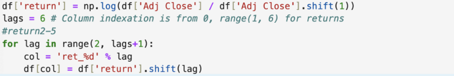
53	Momentum: the trend direction of the stock price is reflected by measuring the rate of change of the stock price. Pt is the current closing price, and Pt – k is the closing price before k, with a general parameter of 6. ${M o m e n t u m}_{t =} P_{t} {- P}_{t - n}$
54-55	Volume Analysis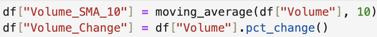

2.2. Target or label definition

The label or the target variable is also known as the dependent variable. Based on experience, developing the following trading strategy:

Selling Strategy: Implement a sell order under any of the following conditions:

The short-term moving average intersects the long-term moving average, indicating a downward trend.

The Relative Strength Index (RSI) exceeds 70, concurrently with the current closing price approaching the upper Bollinger band, signifying an overbought condition.

The Moving Average Convergence Divergence (MACD) line falls below the signal line, suggesting a weakening of momentum.

Buying Strategy: In the absence of the aforementioned conditions, execute a buy order.

Most people are risk-averse and tend to pay more attention to negative returns. Therefore, the final strategy is:

$y_{t} = {\begin{matrix} 0, {\begin{matrix} S M A_s ℎ o r t (t) < S M A_l o n g (t) a n d S M A_s ℎ o r t (t - 1) \geq S M A_l o n g (t - 1) \\ S e l l 2 = R S I (t) > 70 a n d C l o s e (t) \geq B o l l i n g e r U p p e r (t) \\ M A C D (t) < S i g n a l (t) a n d M A C D (t - 1) \geq S i g n a l (t - 1) \end{matrix} \\ 1, O t ℎ e r w i s e \end{matrix}$ (1)

2.3. Transformation

Use a heat map to see correlations between features.

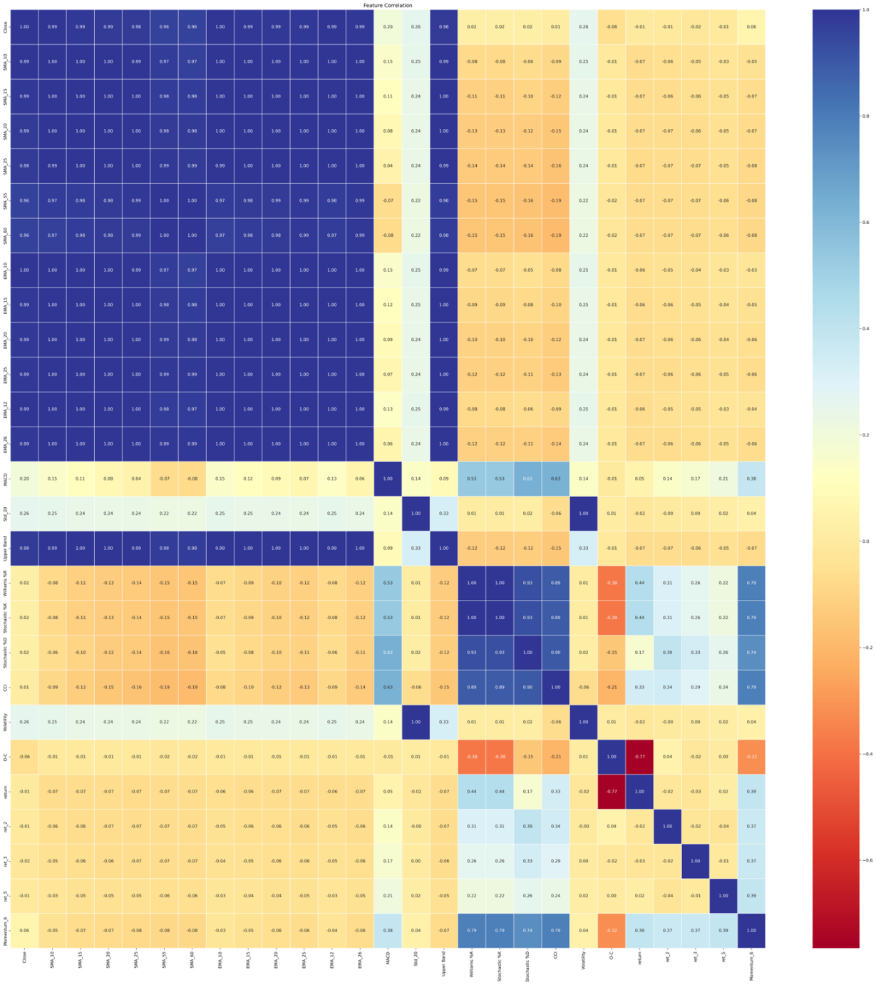
As illustrated in Figure 1, some features exhibit strong correlations, while others are entirely irrelevant. Dimension reduction can reduce the complexity of the model, improve the computational efficiency, help to eliminate noise and improve the generalization ability of the model [9]. In this study, self-organizing mapping (SOM) is used to reduce the dimension, and then principal component analysis (PCA) is used to reduce the dimension of the low-dimensional data output by SOM. SOM dimensionality reduction can preserve the nonlinear topology of data and generate a two-dimensional or three-dimensional representation of low-dimensional space [10]. Building upon the SOM results, PCA is used to further eliminate redundant information and maximize the retention of global variance in the low-dimensional representation. This combined dimensionality reduction approach is particularly effective in handling nonlinear data structures [11].

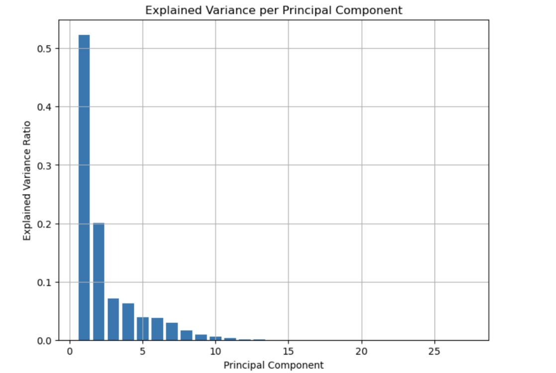
When the number of principal components is set to six, approximately 93% of the total variance in the original dataset can be explained. Principal components beyond this threshold typically contribute minimal additional information and can be discarded. Therefore, the first six principal components are retained to construct the final dataset.

3. Blending modelling

Integrated models can improve the performance and stability of the model, reduce the limitations of a single model and increase the robustness of the model. Blending is an Ensemble Learning approach that uses the prediction results of multiple Base Models as input and then uses a Meta Model to make the final prediction, thereby improving the overall performance of the models [12].

3.1. Selection of the basic model

The Blending algorithm integrates different machine learning algorithms and can make full use of the mathematical principles of each algorithm to learn data from different data Spaces [13]. Therefore, the first-layer classifier of the Blending algorithm should not only have good prediction performance but also have differences among various algorithms. Gradient Boosting and random forest are highly complementary in the integrated model [14]. Gradient Boosting is a serialization algorithm in which subsequent trees rely on the residual adjustment of the previous tree and pay attention to the accuracy of the model. Random forest is a parallel algorithm where each tree is trained independently, focusing on the stability of the model. So, random forest and Gradient Boosting are chosen as base classifiers.

3.2. Selection of the meta-model

Logistic regression is a simple and efficient linear classification model with good interpretability and robustness [15]. The main task of the meta-model is to integrate the predictions of the underlying model. The weights (coefficients) of logistic regression can be regarded as linear weights assigned to the predictions of each underlying model. By learning these weights, logistic regression can dynamically adjust the contribution of the underlying model to the final prediction based on its performance on the validation set, effectively integrating the output of Gradient Boosting and random forest. Logistic regression, as a linear model, complements nonlinear base models such as Gradient Boosting and random forests. Gradient Boosting and random forests are good at capturing complex nonlinear relationships and providing high-quality prediction probabilities. Logistic regression focuses on linear combinations based on these probabilities, avoiding the introduction of further complexity and thus improving the stability of the overall model [15]. Consequently, the second layer uses logistic regression as a meta-learner.

4. Metrics---600

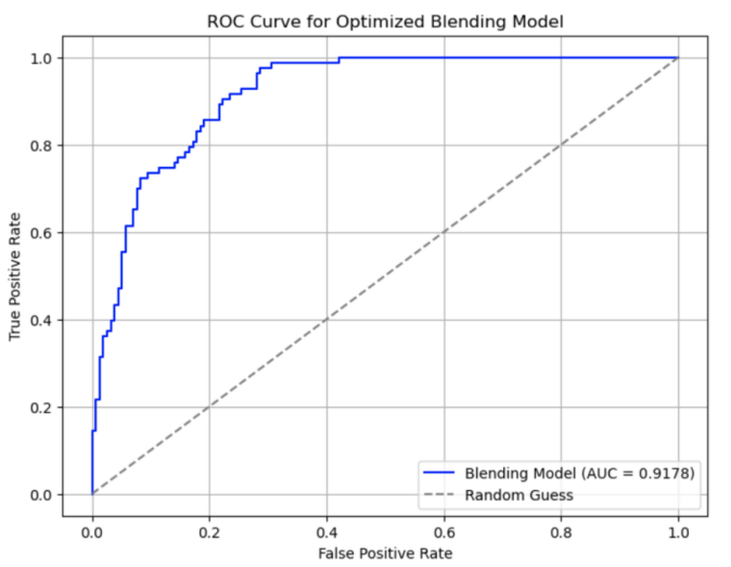
4.1. The area under the ROC curve

The optimized Blending Model achieves excellent classification performance by integrating the prediction results of multiple base models. The performance of AUC = 0.9178 indicates that the model has a significant advantage in the overall classification task and can reliably distinguish positive and negative class samples.

Figure 3. ROC curve for optimized blending model

4.2. Confusion matrix

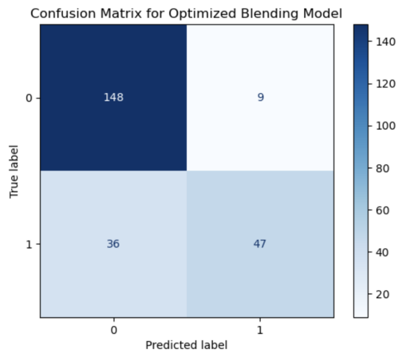
Figure 4. Confusion matrix for optimized blending model

For Class 0, the number of True Negative (148) of negative class samples is significantly higher than that of False Positive (9), indicating that the model makes fewer errors in recognizing negative classes. This makes the model's performance on negative classes very reliable.

For Class 1, the high number of False Negative (36) of positive samples indicates that the model fails to recognize positive samples effectively in some cases. However, 47 True positives indicate that the model still has the capability to predict the Positive class.

4.3. Classification report

In terms of class 0, the model performs well in recognizing category 0andthe Recall rate reaches 0.94, indicating that most samples of category 0 are correctly classified. However, the precision for class 0 is 0.80, indicating that although most class 0 samples are captured, a certain number of negative class samples are misclassified as class 0. Overall, the F1-score of 0.87 for category 0 is a high value, demonstrating that the model's overall performance in this category is excellent. In contrast, the model does not perform as well in class 1 as in class 0. The accuracy rate of class 1 is 0.84, which indicates that the model has good accuracy in predicting class 1. However, the recall rate is only 0.57, which means that a significant number of class 1 samples are not classified correctly. This imbalance between accuracy and recall resulted in the Category 1 F1-score being reduced to 0.68. This difference may be related to an imbalance in the number of class samples - there are significantly more samples in class 0 (157) than in Class 1 (83), making the model more inclined to make correct predictions for class 0.

Table 2. The result of the blending model
Model	Precision (Class 0)	Precision (Class 1)	Recall (Class 0)	Recall (Class 1)	F1-Score (Class 0)	F1-Score (Class 1)	Overall Accuracy
Blending Model	0.80	0.84	0.94	0.57	0.87	0.68	0.80

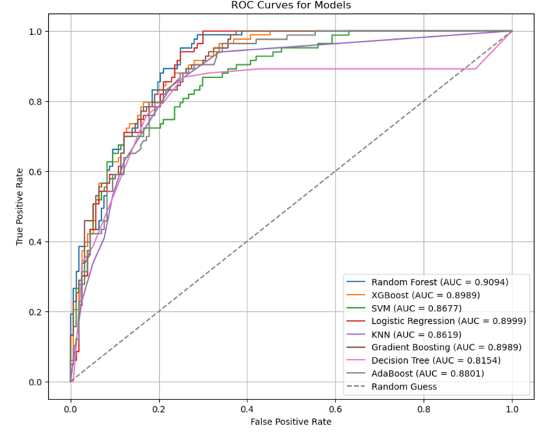
4.4. Comparison with single model

Form table 3, we can clearly see the AUC of the Random Forest model reaches 0.9094, which is the highest among all single models, indicating its strong classification ability. However, its test accuracy is 0.7708, which is slightly lower than other models. The performance of XGBoost and Gradient Boosting is very close, with test accuracy of 0.7917 and 0.7958, respectively and AUC of 0.8989, indicating that the performance of these two models is relatively balanced. The accuracy of the Logistic Regression test was consistent with XGBoost (0.7917) and AUC (0.8999), which also performed well. Blending Model performed best on the test set with a test accuracy of 0.8125, which was significantly higher than that of all single models. Its AUC reached 0.9178, surpassing Random Forest's AUC of 0.9094 and other models. This indicates that the Blending Model is stronger in the overall classification ability and the ability to distinguish positive and negative samples.

Table 3. The result of the single models
	Testing Accuracy	AUC
Random Forest	0.770833	0.909447
XGBoost	0.791667	0.898933
SVM	0.758333	0.867738
Logistic Regression	0.791667	0.899931
KNN	0.775000	0.861945
Gradient Boosting	0.795833	0.898933
Decision Tree	0.754167	0.815402
AdaBoost	0.766667	0.880055
Blending Model	0.8125	0.9178

Compared with a single Model, the Blending Model effectively improves the test accuracy and AUC by integrating the prediction results of multiple base models (Gradient Boosting and Random Forest). This enhancement shows that the Blending Model combines the advantages of different models and overcomes the limitations of a single model. Especially on the AUC index, the performance of the Blending Model further strengthens its stability and its ability to distinguish samples. In a single model, although the AUC of Random Forest is higher, its test accuracy is lower and there may be some bias. The linear combination of the Blending Model reduces the impact of similar problems through weight distribution.

Table 4. Comparison between a single model and a hybrid model
Model	Precision (Class 0)	Precision (Class 1)	Recall (Class 0)	Recall (Class 1)	F1-Score (Class 0)	F1-Score (Class 1)	Overall Accuracy	False Negatives (Class 1)
Gradient Boosting	0.80	0.77	0.91	0.58	0.85	0.66	0.80	35
Logistic Regression	0.80	0.78	0.92	0.55	0.85	0.65	0.79	37
Random Forest	0.77	0.79	0.94	0.46	0.84	0.58	0.77	45
Blending Model	0.80	0.84	0.94	0.57	0.87	0.68	0.81	36

It can be seen from Table 4 that:

· Class 0 and Class 1 Performance:

The Blending Model achieves the highest Precision (Class 1) at 0.84, outperforming all single models, indicating better accuracy in predicting positive samples.

Its Recall (Class 1) at 0.57 is better than Logistic Regression and Random Forest but slightly lower than Gradient Boosting.

· F1-Score:

The Blending Model's F1 Score (Class 1) is 0.68, the best among all models. It showcases balanced performance in precision and recall.

For Class 0, the Blending Model also achieves the highest F1-Score at 0.87, indicating superior performance in negative sample classification.

· Overall Accuracy:

The Blending Model achieves the highest overall accuracy at 0.81, surpassing Gradient Boosting (0.80) and Logistic Regression (0.79).

·False Negatives (Class 1):

The Blending Model reduces the number of false negatives for Class 1 to 36, significantly better than Random Forest (45) and comparable to Gradient Boosting (35).

The table clearly shows that the Blended Model outperforms single models in terms of Class 1 Precision, Class 1 F1 Score, and overall accuracy while maintaining competitive performance in reducing false negatives for Class 1. By integrating the strengths of Gradient Boosting and Random Forest, the Blended Model demonstrates superior overall classification performance.

5. Conclusion

This paper investigates stock movement trend prediction using daily trading data from AAPL, proposing a prediction framework based on the Blending ensemble learning algorithm. Initially, the single classification algorithm is used for prediction and the prediction effect of each algorithm is analysed under the dimensions of AUC and the accuracy evaluation index. Then, the correlation between each algorithm is comprehensively considered and the algorithm of "good but different" is selected as the base classifier of the first layer of the Blending algorithm. Based on the principle of combining models that are both effective and diverse, Gradient Boosting and Random Forest were selected as the base classifiers in the first layer of the Blending framework. The predictions from these base models were then used to construct a new dataset, which was further processed by a Logistic Regression model serving as the meta-classifier to generate the final prediction. Experimental results demonstrate that the Blending model, incorporating Gradient Boosting and Random Forest as base learners and Logistic Regression as the meta-learner, achieves superior performance in stock trend prediction compared to individual models.

To further improve the performance of the Blending model, the decision threshold can be adjusted to improve the sensitivity to class 1 and capture more positive trend signals. Additionally, incorporating class weighting during training could better address class imbalance by increasing the penalty for misclassifying minority class samples. Expanding the feature set and applying feature selection techniques may also help reduce noise and improve model efficiency.

In future work, the selection and combination of classifiers will be further discussed. This study primarily focused on two classical algorithms; however, the inclusion of additional or more advanced models as base learners could further enrich the Blending framework and improve predictive performance.

References

[1]. BASAK S, KAR S, SAHA S, et al(2019). Predicting the direction of stock market prices using tree⁃based classifiers [J]. The North American journal of economics and finance, 47: 552-567.

[2]. CHEN Y J, HAO Y T(2017). A feature weighted support vector ma⁃ chine and K⁃nearest neighbor algorithm for stock market indices prediction [J]. Expert systems with applications, 80: 340-355.

[3]. Feng, H. (2024) A Blended Teaching Model of College English Based on Deep Learning. Journal of Electrical Systems. [Online] 20 (6s), 1505-1515.

[4]. Ficuciello, F. & Siciliano, B. (2016) Learning in robotic manipulation: The role of dimensionality reduction in policy search methods: Comment on “Hand synergies: Integration of robotics and neuroscience for understanding the control of biological and artificial hands” by Marco Santello et al. Physics of life reviews. [Online] 1736-37.

[5]. PATEL J, SHAH S, THAKKAR P, et al(2015). Predicting stock and stock price index movement using trend deterministic data preparation and machine learning techniques [J]. Expert systems with applications, 42(1): 259⁃268.

[6]. CHEN Y J, HAO Y T(2017). A feature weighted support vector ma⁃ chine and K⁃nearest neighbor algorithm for stock market indices prediction [J]. Expert systems with applications, 80: 340-355.

[7]. BASAK S, KAR S, SAHA S, et al(2019). Predicting the direction of stock market prices using tree⁃based classifiers [J]. The North American journal of economics and finance, 47: 552-567.

[8]. RODRíGUEZ⁃GONZáLEZ A, GARCíA⁃CRESPO Á, COLOMO⁃ PALACIOS R, et al(2011). CAST: using neural networks to im⁃ prove trading systems based on technical analysis by means of the RSI financial indicator [J]. Expert systems with applica⁃ tions, 38(9): 11489-11500.

[9]. Ficuciello, F. & Siciliano, B. (2016) Learning in robotic manipulation: The role of dimensionality reduction in policy search methods: Comment on “Hand synergies: Integration of robotics and neuroscience for understanding the control of biological and artificial hands” by Marco Santello et al. Physics of life reviews. [Online] 1736–37.

[10]. Xia, B. et al. (2019) Using Self Organizing Maps to Achieve Lithium-Ion Battery Cells Multi-Parameter Sorting Based on Principle Components Analysis. Energies (Basel). [Online] 12 (15), 2980-.

[11]. Hiremath, V. et al. (2011) Combined dimension reduction and tabulation strategy using ISAT–RCCE–GALI for the efficient implementation of combustion chemistry. Combustion and flame. [Online] 158 (11), 2113–2127.

[12]. López-Cuesta, M. et al. (2023) Improving Solar Radiation Nowcasts by Blending Data-Driven, Satellite-Images-Based and All-Sky-Imagers-Based Models Using Machine Learning Techniques. Remote sensing (Basel, Switzerland). [Online] 15 (9), 2328-.

[13]. Feng, H. (2024) A Blended Teaching Model of College English Based on Deep Learning. Journal of Electrical Systems. [Online] 20 (6s), 1505–1515.

[14]. Sandhu, A. K. & Batth, R. S. (2021) Software reuse analytics using integrated random forest and gradient boosting machine learning algorithm. Software, practice & experience. [Online] 51 (4), 735–747.

[15]. Mojsilovic, A. (2005) 'A logistic regression model for small sample classification problems with hidden variables and non-linear relationships: an application in business analytics’, in Proceedings. (ICASSP ’05). IEEE International Conference on Acoustics, Speech, and Signal Processing, 2005. [Online]. 2005 IEEE. p. v/329-v/332 Vol. 5.

[16]. Merlo, J. et al. (2016) An Original Stepwise Multilevel Logistic Regression Analysis of Discriminatory Accuracy: The Case of Neighbourhoods and Health. PloS one. [Online] 11 (4), e0153778–e0153778.

Cite this article

Li,X. (2025). Application of Blending-based Ensemble Algorithm in Stock Prediction. Applied and Computational Engineering,178,292-303.

Data availability

The datasets used and/or analyzed during the current study will be available from the authors upon reasonable request.

Disclaimer/Publisher's Note

The statements, opinions and data contained in all publications are solely those of the individual author(s) and contributor(s) and not of EWA Publishing and/or the editor(s). EWA Publishing and/or the editor(s) disclaim responsibility for any injury to people or property resulting from any ideas, methods, instructions or products referred to in the content.

About volume

Volume title: Proceedings of CONF-CDS 2025 Symposium: Data Visualization Methods for Evaluatio

ISBN：978-1-80590-285-0(Print) / 978-1-80590-286-7(Online)

Editor：Marwan Omar, Elisavet Andrikopoulou

Conference website: https://2025.confcds.org/portsmouth.html

Conference date: 30 July 2025

Series: Applied and Computational Engineering

Volume number: Vol.178

ISSN：2755-2721(Print) / 2755-273X(Online)

© 2024 by the author(s). Licensee EWA Publishing, Oxford, UK. This article is an open access article distributed under the terms and conditions of the Creative Commons Attribution (CC BY) license. Authors who publish this series agree to the following terms:
1. Authors retain copyright and grant the series right of first publication with the work simultaneously licensed under a Creative Commons Attribution License that allows others to share the work with an acknowledgment of the work's authorship and initial publication in this series.
2. Authors are able to enter into separate, additional contractual arrangements for the non-exclusive distribution of the series's published version of the work (e.g., post it to an institutional repository or publish it in a book), with an acknowledgment of its initial publication in this series.
3. Authors are permitted and encouraged to post their work online (e.g., in institutional repositories or on their website) prior to and during the submission process, as it can lead to productive exchanges, as well as earlier and greater citation of published work (See Open access policy for details).