1. Introduction

Machine learning is a hot and universal topic in nowadays technology field. Artificial intelligence (AI) can be applied to field like bioinformatics, fraud detection, finical market analysis, image recognition and natural language processing (NLP) based on machine learning [1]. Deep learning is a type of machine learning with multiple layers. Image recognition is a filed highly based on CNN. When CNN is used to specific image classification regions, with different CNN models, AI can be trained to reach a high accuracy for putting things into different categories. For typical classification tasks like dogs and cats, accuracy is implemented to be over 94% [2].

For deep learning, basically three main types of training methods are included, supervised learning, unsupervised learning and semi-supervised learning [1]. Usually, image classification provides distinct categories for different inputs, which in case is supervised learning. Based on standard output, computer automatically calculate mathematical relations between input and output. Error in loss function is backpropagated to adjust these mathematical relations.

CNN is a typical deep learning architecture. Along the development of CNN, various algorithms are applied to optimize its output accuracy and model size. In this article, facemask detection is implemented based on five models in CNN: AlexNet, VGG, ResNet, EfficienNet and Vit.

Facemask detection is universally applied in epidemic period for safety concern and saving of manpower resource. In public places, established camera facing problems like long-term using and environment intrusion. Electronic circuits heat for long-term running, producing Gaussian white noise like thermal noise. Long-term using also influence camera sensor sensitivity and analog to digital converter (ADC), giving noise like salt and pepper. Environment intrusion like extreme light condition creates gaussian white noise. Electromagnetic interferences in the environment create impulse noise.

Gaussian noise and impulse noise are compounded into pictures to simulate noise condition. CNN models are training with pure images. Anti-interference ability of noise is tested by observing model accuracy with input of noisy images. This ability is important for model selection in practical condition, giving appropriate facility establishment and recourse saving.

Model part introduced features of selected CNN models. Method part gives training instructions and testing procedures of anti-interference ability. Model performances are summarized and compared in result part.

2. Model

CNNs are inspired by human brain biological processes. Connectivity inside human brain’s visual cortex is what CNN designed to mimic. Compared with conventional neural network, CNN performs convolution layers with two main attributes: sparse interactions and parameter sharing [1]. Sparse interaction is designed to apply smaller kernels. Total parameters in computing process are reduced, making better memory utilization. Parameter sharing represents weights sharing. While working on different receptive fields, filter possess same group of weights to abstract features.

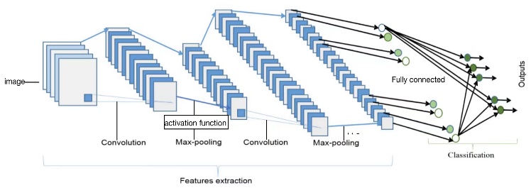
Figure 1. Whole process for CNN. Feature extraction process includes convolution layer, activation function and pooling.

CNNs for classification jobs possess three working blocks which is shown in figure 1 [3]. First, with convolution layers, picture features of different regions will be extracted through multiplication between pixels and kernels. These kernels (filters) are matrix with different combination of weights for functions like blurring, sharping or edge detection [4].

In second block, Pooling layer receives feature map from previous layer, making down sampling of it. Inside each pooling window, function generates a representative value over statistical values [1,3]. Max pooling, average pooling are universal pooling functions adopted in CNN algorithms.

Convolution layer and pooling layer are linear process. Outputs from these layers do not satisfy requirement of classification. Activation function is applied to infer non-linear feature map. Selection is based on input data and requirement of output region. Representative activation function includes sigmoid, ReLU, etc.

These three blocks are not necessarily in sequential. Constructing CNNs by giving reasonable combinations of them. Different models vary in feature extraction step, combination of working blocks. Blocks vary in selection of activation function, kernel size, layer amount, etc.

2.1. AlexNet

AlexNet is a CNN structure with eight learning layers, five of which are convolution layer and rest are fully connected. For original AlexNet network, two GPU are applied for calculation. It can be converted into single GPU version with entire structure shown in figure 2 [5].

Three max-pooling layers with size of 3×3 is separately applied after first, second and fifth convolution layer [5]. Activation function of ReLU is applied after each convolution layer. For standard input image, 96 kernels with size of 11×11×3 are applied in first layer. Second layer takes 256 kernels with size of 5×5×96. Kernels inside third, fourth and fifth layers are with size of 3×3, but with different depth of 256, 384 and 384. Number of kernels for last three convolution layers are 384, 384 and 256. Fully connected layers are with 4096 neurons of each and provide inputs to a 1000-way softmax classifier [5, 6].

2.2. VGG

Compare with AlexNet, VGG applies filers with smaller respective filed which is mainly 3×3 and partially 1×1. Application of smaller filter reduce total parameters produced along convolution process. Selecting VGG16 to represent and fully structure is shown in figure 2 [7].

ReLU is connected to hidden layer as activation function for non-linearity. Max-pooling layers at end of each convolution group are equally with window size of 2×2. All convolution layers inside VGG16 share the same respective filed size of 3×3 for each kernel. From first to fifth group, 64, 128, 256, 512 and 512 are filter numbers for convolution layers. First and second group have two convolution layers and rest groups have three layers inside. Configurations for following part of VGG are the same with AlexNet [6, 7].

2.3. ResNet

Theoretically, solving of over-fitting problem guarantees increasement of model accuracy while the increasement of layers [8]. Problems like vanishing gradient and degradation occurs for multiple layers being applied to architectures like AlexNet and VGG [9]. In ResNet configuration, concept of residual is induced for optimization of these problems. Structure of ResNet18 is shown in figure2 as representation of residual network [9].

ResNet applies batch normalization (BN) to avoid over-fitting. Convolution layers inside ResNet are divided into 5 groups. From second group to last one, numbers of filters increase from 64 to 512 with each time multiplying 2 [9]. Down sampling process divide size of feature map by two, shown as “/2” in figure 2 [3,9]. Two convolution blocks exist in each convolution group of ResNet18. Residual is applied each time data pass through one convolution block, showing in line. Dash line means down sampling of shortcut [9]. Respective field is applied with stable size of 3×3. Ending configuration is consisted by an average pooling and a 1000-way softmax classifier [9].

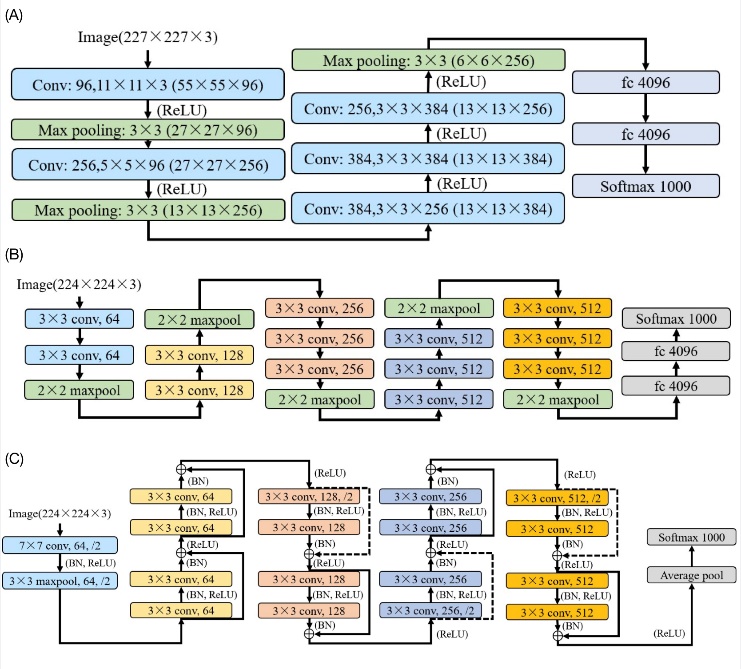
Figure 2. Model structure of CNNs with details of hidden layers and activation function. (A): AlexNet structure. (B): VGG 16 structure. (C): ResNet 18 structure.

2.4. EfficientNet

Concept of residual network is invented in ResNet. MobileNet offers a relative concept of inverted residual network. Residual network gives operation for channel to change from wide to narrow and back to wide. Inverted residual network operates oppositely, changing channel from narrow to wide and back to narrow [10]. This inverted residual network is MBConv block.

A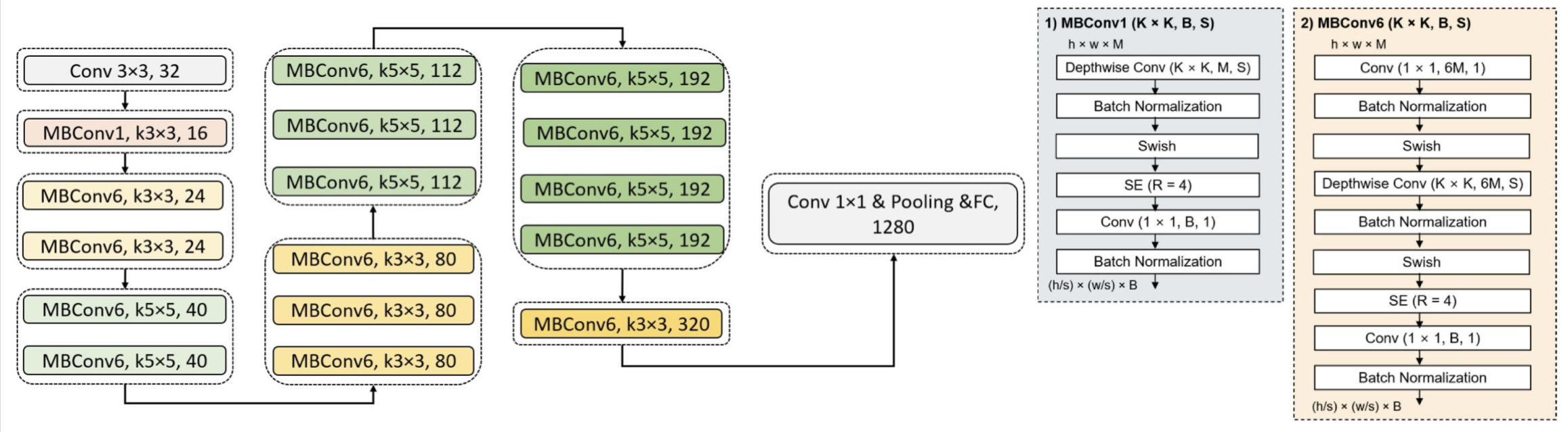

B

Figure 3. A is main structure of Effb0. B gives exact operation inside MBConv1 and MBConv6.

In EfficientNet, this MBConv is highly applied for model configuration. Select Effb0 as representation. Figure 3 shows structure for Effb0, MBConv1 and MBConv6 [11, 12]. Effb0 is constructed by nine stages of operation. First stage is normal convolution layer with kernel size of 3×3. Last stage is operation with fully connected layer and classifier. Other stages are combinations of MBConv blocks with different channels. Stage information is shown in figure 3 with amount and kernel size. Each dash line block means one stage.

2.5. Vision transformer

Vision transformer is not a typical CNN model. Concept of attention is introduced into image processing area through Vit. Core of Vit is processed based on encoder part in original transformer [13]. Detail for encoder is shown in figure 4. Universally encoder include two sublayers, self-attention and position-wise feed forward neural network (FFNN) [14]. Multi-headed attention enable computer to be conscious of relationship among different part of inputs. MLP or FFNN includes two linear transformations with ReLU activation in between. Layernorm and residual is applied in encoder block.

Figure 4 gives universal structure for Vit. Image is split based on input batch size, multiplying with an embedding matrix. Giving final Vit input by fusing position vector. Input batch size is 16×16 for selected Vitb16 [14]. Layers in encoder contain linear projection mapping of flatten patches of dimension D refined during training. This D parameter equal to 768 for selected Vitb16 structure [14].

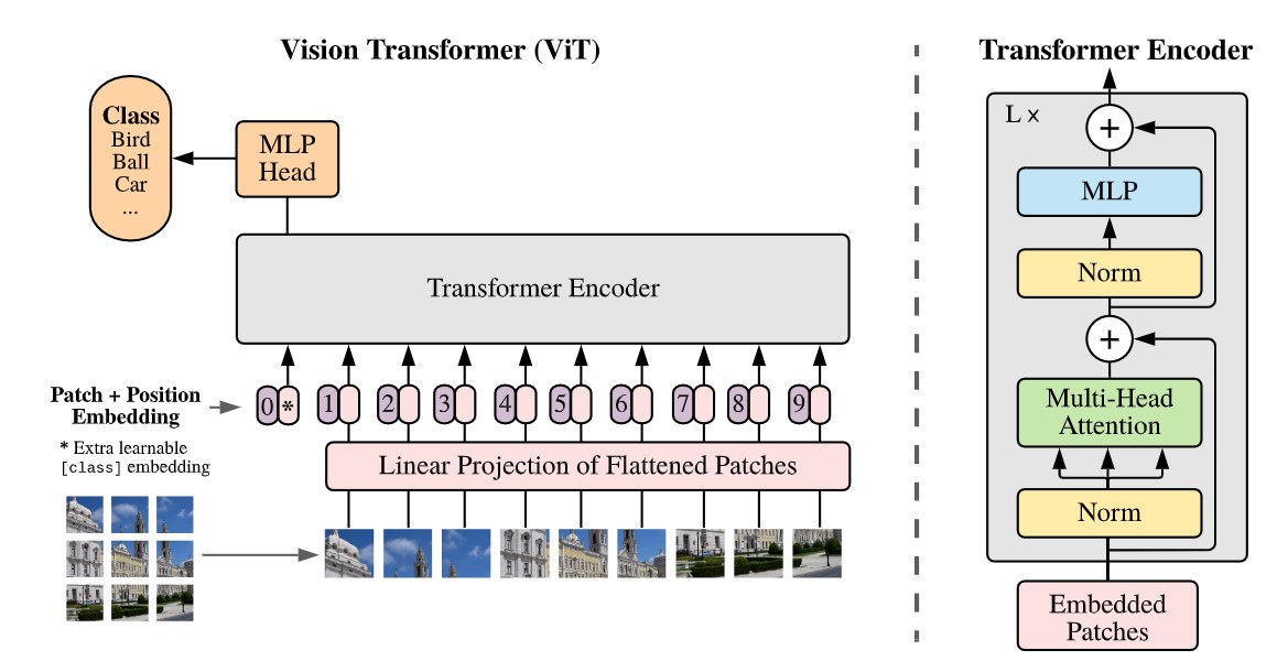
Figure 4. Left: universal structure for Vit. Right: encoder

3. Method

Dataset with train, validation and test parts is applied for CNN model establishment. Source of this dataset is from Kaggle [15]. Images in each part of the dataset are divided into two categories, WithMask and WithoutMask. Import relative CNN models from PyTorch library [16]. Modify input images and model classifier to obtain similar condition for anti-interference testing. Establishing complete deep learning process by adding relevant loss function and optimizer.

3.1. Preprocessing

3.1.1. Input resizing. Before training of CNN model, image resizing is implemented based on image processing function of OpenCV. Based on torchvision.model [16], all images are reshaped to size of 224×224. Resizing aims to keep input parameter balancing for training and testing.

3.1.2. Noise adding. To test anti-interference ability of CNN, processing original test images by adding gaussian noise, impulse noise and their combination. Gaussian noise is added to each pixel of images, their value conforms gaussian distribution. Method to control noise level is changing variance of gaussian distribution, considering mean value of 0 [17]. Impulse noise randomly appears on images with pixels like sale and pepper. Changing its level by applying different noise density. Setting variance of gaussian noise in range from 1 to 50 and noise density of impulse noise in range from 0.001 to 0.05 [18]. Increasing noise level with step 1 for Gaussian and step 0.001 for Impulse. Then apply combined noise to images for more practical condition. Totally 150 groups of new test images are generate based on different noise level.

3.1.3. Model changing. Classifier for original models is 1000-way softmax, distinguishing 1000 categories. Only two categories exist in facemask classification. Changing fully connected layers before softmax into two down-sampling layers. Linking sigmoid activation function instead of softmax for classification of two categories.

3.2. Training

All the hyperparameters are the same for each kind of model training, making comparisons of model being less affected by things out of model itself. Applying precisely cross validation to ensure reasonable hyperparameters.

Train part of dataset contains 10,000 images in total for two categories. Validation part contains 800 in total. Setting start number of batch size. In each epoch, inputting validation images into model after training of all train images. This step aims to observe whether model is over-fitting or not. With increment of epoch, stop training once over-fitting occurs and record the batch size with epoch. Change batch size, redo these operations to have a new group of recording. Repeat training and validation with same process for selected models. Selecting group of hyperparameters for tradeoff of all model’s performance.

3.3. Model updating

Backpropagation refreshes weights on each neural of CNN, giving better performance of overall model. Loss function and optimizer is responsible for this process. Again, same loss function and optimizer is selected for all models to control variable.

Mask detection task is a binary classification task. After sigmoid activation function at end of CNN model, binary cross entropy loss (BCEloss) function is applied for loss calculation. Data after BCEloss goes into optimizer for weights adjustment. Adaptive moment estimation (Adam) is selected optimizer for weights refreshing.

Final step is to upgrade model in each epoch of training. Comparisons between losses are made. Once output loss is smaller than the previous one, weights inside the model is recorded for model updating. Model with relatively best performance is established after running all training epochs.

3.4. Testing

Recognizing accuracy is parameter representing model’s anti-interference ability of noise. After model training and establishing, putting test dataset with different noise level to generate relative recognizing accuracy. Recording accuracy number of different noise level for comparison.

4. Results and discussion

4.1. Prepocesssed images

Images preprocessed with noise is shown in figure 5. Selecting of 6 specific points. Gaussian noise variance is at 1, 10, 20, 30, 40 and 50. Impulse noise with density at 0.001, 0.01, 0.02, 0.03, 0.04 and 0.05. Noise combination is at the pattern of 1 and 0.001 and so on.

Accuracies for mainstream models are high under ideal condition. In table 1, nearly 100 percent for all models, making no difference for recognizing result. With similar recognizing performance, model dominance can be generated from recognizing time. In table 1, AlexNet and ResNet18 holds the shortest recognizing time. This running time is similar for noisy image testing.

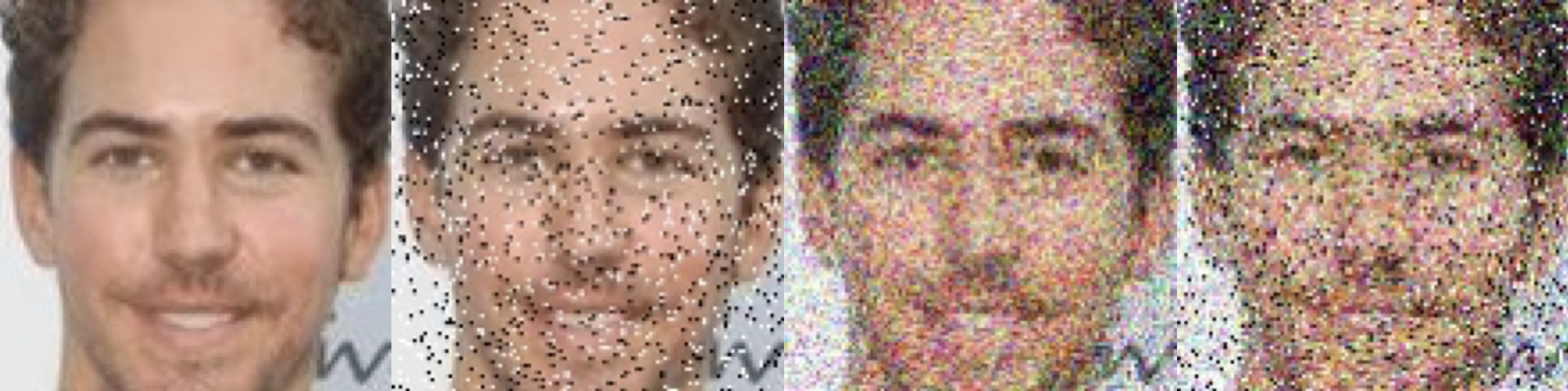
Figure 5. Preprocessed images with noise. From left to right, pure, impulse noise, gaussian noise and mixed noise.

4.2. Test result with pure images (No Noise)

Table1. Ideal condition.

4.3. Comparision for noisy images

In figure 6, accuracies for recognizing noisy images of five models are shown in line graph. This figure separately gives three accuracy graphs, showing results for pure gaussian noise, pure impulse noise and mixed noise of these two kinds. In each graph, five accuracy lines of different colors are plotted, representing five models. Generating model anti-interference ability of noise by observing and comparing line moving tendency in these graphs.

A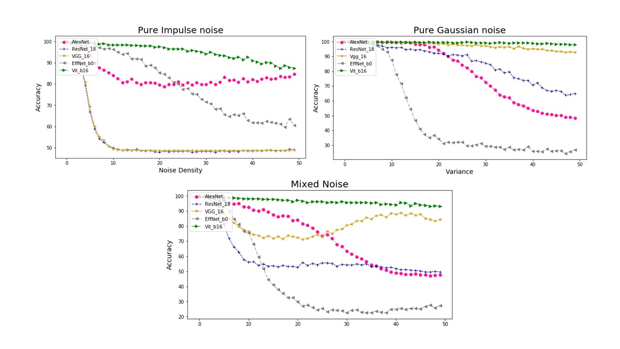

B

C

Figure 6. Three graphs representing model accuracy under practical cameral condition. A is pure salt and pepper noise. B is pure gaussian noise and C is mixture of these two kinds.

Observing figure 6 in whole, most of models possessing a directly accuracy changing when noise level rise from unit amount to 20 times of it. Accuracy line goes flatten after 20 times of unit noise level. Hypothesis can be generated from this general outcome. When noise level goes inside a certain range, several features are more distinguishable for CNN in the picture. For example, in figure 5, eyes of human are distinct under high noise level.

To generate model anti-interference ability of noise, comparing each line inside certain accuracy graph.

4.3.1. Pure gaussian noise. Recognizing ability for VGG16 and Vitb16 has nearly not be affect for gaussian noise. AlexNet possess better accuracy than ResNet18 before gaussian noise variance goes up to 20. ResNet18 has accuracy downing like small slope linear process. AlexNet has accuracy downing like reversed sigmoid function. Accuracy of EffNetb0 quickly decreases to 30 percent when gaussian variance rise to around 15.

For pure gaussian noise, VGG and vision transformer have high anti-interference ability. EffNet gives terrible tolerance of gaussian noise. AlexNet and ResNet can be established for low level gaussian noise.

4.3.2. Pure impluse noise. Vitb16 possess accuracy within 90 percent for entire noise levels. VGG16 and ResNet18 recognizing ability rapidly attenuate to 50 percent for noise density increased to 0.01. AlexNet accuracy downs to around 80 percent at 0.01. Unexpectedly, AlexNet accuracy increases for higher noise density. EffNetb0 accuracy moves from 99 to around 60, possessing linear downing curve.

Generating model anti-interference ability of impulse noise. Vision transformer is stable and accurate for whole test noise range. VGG and ResNet are not acceptable for recognizing purely impulse noise. AlexNet acts well for extreme level of impulse noise. EffNet is acceptable with noise density under 0.02.

4.3.3. Mixed noise. Vitb16 possesses accuracy within 90 percent for entire noise level. Below 25 times of unit noise level, AlexNet has recognizing accuracy above 80 percent. Then, it goes flatten around 50 percent for noise level over 35 times of unit. Accuracy for ResNet18 rapidly downs to 50 percent at 10 time of unit noise level. A flatten accuracy line occurs for rest testing noise level. Accuracy for EffNetb0 drops for three stages. First stage to 80 percent at 10 times unit noise level, second to 30 percent at 20 times unit noise level and goes flatten near 25 percent for the rest. VGG16 curve gives most unexpected result. It quickly drops to 80 percent at 10 times of unit noise level and goes flatten until 20 times. An increasing recognizing accuracy occurs for VGG16 when noise level increases from 20 times to 35 percent, and stable at 90 percent from 35 times to 50 times.

5. Conclusion

In a nutshell, Vision Transformer gives best performance for all test condition with a relevant running speed. AlexNet gives similar accuracy line for each tested noise, giving a qualified accuracy for high level of pure impulse noise. VGG is skilled in recognizing gaussian noise. It also obtains high level anti-interference ability for mixed noise. Running time is too long compare with other models. ResNet gives relatively equivalent accuracy for each kind of noise. EfficientNet possess anti-interference ability for impulse noise in a little range. Its accuracy line drops steeply for gaussian and mixed noise.

This article only included limited model types and amount of dataset. Only one architecture is selected from each model. All the above limitations are required to broaden up to obtain noise anti-interference ability more precisely.

References

[1]. W. Pedrycz and S.-M. Chen, Deep learning : concepts and architectures / edited by Witold Pedrycz, Shyi-Ming Chen. Cham, Switzerland : Springer, 2020.
[2]. B. Liu, Y. Liu, and K. Zhou, "Image classification for dogs and cats," TechReport, University of Alberta, 2014.
[3]. M. Z. Alom et al., "The history began from alexnet: A comprehensive survey on deep learning approaches," arXiv preprint arXiv:1803.01164, 2018.
[4]. J. P. Mueller and L. Massaron, Deep Learning for dummies. John Wiley & Sons, 2019.
[5]. A. Krizhevsky, "One weird trick for parallelizing convolutional neural networks," arXiv preprint arXiv:1404.5997, 2014.
[6]. W. Yu, K. Yang, Y. Bai, T. Xiao, H. Yao, and Y. Rui, "Visualizing and comparing AlexNet and VGG using deconvolutional layers," in Proceedings of the 33 rd International Conference on Machine Learning, 2016.
[7]. K. Simonyan and A. Zisserman, "Very deep convolutional networks for large-scale image recognition," arXiv preprint arXiv:1409.1556, 2014.
[8]. V. Atliha and D. Šešok, "Comparison of VGG and ResNet used as Encoders for Image Captioning," in 2020 IEEE Open Conference of Electrical, Electronic and Information Sciences (eStream), 2020: IEEE, pp. 1-4.
[9]. K. He, X. Zhang, S. Ren, and J. Sun, "Deep residual learning for image recognition," in Proceedings of the IEEE conference on computer vision and pattern recognition, 2016, pp. 770-778.
[10]. M. Sandler, A. Howard, M. Zhu, A. Zhmoginov, and L.-C. Chen, "Mobilenetv2: Inverted residuals and linear bottlenecks," in Proceedings of the IEEE conference on computer vision and pattern recognition, 2018, pp. 4510-4520.
[11]. M. Tan and Q. Le, "Efficientnet: Rethinking model scaling for convolutional neural networks," in International conference on machine learning, 2019: PMLR, pp. 6105-6114.
[12]. S. Gang, N. Fabrice, D. Chung, and J. Lee, "Character Recognition of Components Mounted on Printed Circuit Board Using Deep Learning," Sensors, vol. 21, no. 9, p. 2921, 2021.
[13]. A. Dosovitskiy et al., "An image is worth 16x16 words: Transformers for image recognition at scale," arXiv preprint arXiv:2010.11929, 2020.
[14]. S. Gkelios, Y. Boutalis, and S. A. Chatzichristofis, "Investigating the vision transformer model for image retrieval tasks," in 2021 17th International Conference on Distributed Computing in Sensor Systems (DCOSS), 2021: IEEE, pp. 367-373.
[15]. A. JANGRA. Face Mask Detection ~12K Images Dataset [Online] Available: https://www.kaggle.com/datasets/ashishjangra27/face-mask-12k-images-dataset/download
[16]. Torch. "MODELS AND PRE-TRAINED WEIGHTS." https://pytorch.org/vision/stable/models.html (accessed 10, 4, 2022).
[17]. A. C. Bovik, The essential guide to image processing. Academic Press, 2009.
[18]. L. Navarro, G. Courbebaisse, and M. Jourlin, "Chapter Two - Logarithmic Wavelets," in Advances in Imaging and Electron Physics, vol. 183, P. W. Hawkes Ed.: Elsevier, 2014, pp. 41-98.
Cite this article
Huang,W. (2023). Anti-inference ability of CNN mainstream models based on face mask detection. Applied and Computational Engineering,2,294-303.
Data availability
The datasets used and/or analyzed during the current study will be available from the authors upon reasonable request.
Disclaimer/Publisher's Note
The statements, opinions and data contained in all publications are solely those of the individual author(s) and contributor(s) and not of EWA Publishing and/or the editor(s). EWA Publishing and/or the editor(s) disclaim responsibility for any injury to people or property resulting from any ideas, methods, instructions or products referred to in the content.
About volume
Volume title: Proceedings of the 4th International Conference on Computing and Data Science (CONF-CDS 2022)
© 2024 by the author(s). Licensee EWA Publishing, Oxford, UK. This article is an open access article distributed under the terms and
conditions of the Creative Commons Attribution (CC BY) license. Authors who
publish this series agree to the following terms:
1. Authors retain copyright and grant the series right of first publication with the work simultaneously licensed under a Creative Commons
Attribution License that allows others to share the work with an acknowledgment of the work's authorship and initial publication in this
series.
2. Authors are able to enter into separate, additional contractual arrangements for the non-exclusive distribution of the series's published
version of the work (e.g., post it to an institutional repository or publish it in a book), with an acknowledgment of its initial
publication in this series.
3. Authors are permitted and encouraged to post their work online (e.g., in institutional repositories or on their website) prior to and
during the submission process, as it can lead to productive exchanges, as well as earlier and greater citation of published work (See
Open access policy for details).