1. Introduction

Tropical cyclones, also known as typhoons in the Western Pacific, hurricanes in the Atlantic, and cyclones in the Indian Ocean, are among the most destructive natural hazards. They bring extreme rainfall and damaging winds and regularly cause substantial loss of life and property in coastal regions. Notable recent disasters include Typhoon Haiyan (2013), which caused over 6,000 deaths, and Typhoon Yagi (2024), which caused about 300 deaths in Vietnam [1,2]. Timely, skillful forecasts can reduce exposure, guide evacuations, and optimize emergency resource allocation [3,4]. Therefore, accurate and timely prediction is essential to mitigate losses.

In recent years, artificial intelligence (AI) has shown strong performance in learning complex, nonlinear relationships from high-dimensional spatiotemporal data, enabling data-driven forecasting and decision support in geoscience and beyond. Many machine-learning models have been applied to natural-disaster prediction, including earthquakes and floods [5-8]. Mosavi et al. highlighted the role of neural networks in estimating flood peak [7]. For earthquakes, Asim et al. proposed a hybrid model that demonstrated global predictive skill [8]. More recently, Buch et al. simulated wildfire frequency in the western U.S. using the SML Fire 1.0 model [9]. Compared with traditional statistical approaches, AI methods can improve intensity and impact predictions by efficiently learning from historical tracks and temporal evolution of past events.

Typhoons remain a central challenge in atmospheric science. In 2008, Jin et al. developed a nonlinear AI ensemble for forecasts in the South China Sea, addressing overfitting common to earlier neural networks [10]. Decades later, Meng et al. introduced a probabilistic machine-learning model for tropical-cyclone intensity with calibrated uncertainty [11], and Liu et al. integrated the Pangu machine-learning model with the WRF numerical weather prediction system [12]. Xu et al. has taken a deep learning approach using convolutional neural network [13]. These studies highlight significant progress. Nevertheless, multi-day track prediction remains difficult under highly variable environmental forcing, and institutional adoption can be hampered by trust, interpretability, and operational integration constraints.

This study employs and evaluates three machine learning models for 24-hour-advanced peak-intensity prediction using a parsimonious, pre-peak track representation augmented with simple covariates. Our goal is to assess how far track-centric, tabular AI can go in forecasting maximum intensity, and to clarify its operational value as a fast, transparent baseline that can complement more data-intensive approaches and support preparedness and response planning.

2. Method

We conducted a retrospective, observational modeling study using historical best-track records of Western North Pacific tropical cyclones to develop and compare data-driven predictors of peak intensity 24 hours in advance. The approach frames intensity forecasting as supervised learning on standardized pre-peak track histories augmented with a small set of readily available covariates. We benchmarked a simple linear model against modern nonlinear learners to assess the value of capturing interactions and nonlinearity, and we evaluated models with complementary accuracy and calibration metrics on a temporally held-out cohort to approximate prospective generalization. To probe robustness and operational relevance, we stratified errors across climatologically meaningful groups (seasonality, latitude, and intensity class) and employed interpretable machine learning tools to summarize feature contributions. All analyses were implemented in Python using widely adopted machine-learning libraries.

2.1. Data

The data of past typhoons were extracted from ibtracs.com and filtered out the newest 400 typhoons from 2012 to 2025 to ensure the quality of the data. The data contains time, location, and intensity-related data recorded by multiple meteorological agencies, including the Japan Meteorological Agency (JMA) and the Joint Typhoon Warning Center (JTWC) at Pearl Harbor. For each typhoon, the data is recorded every three hours.

2.2. Targets and predictors

For each typhoon, we identified the maximum wind speed and the minimum pressure as the peak intensity. Because storms have various lifetimes, only 37 coordinates of the track to 24 hours prior to the peak intensity were kept and used as features of latitudes and longitudes, corresponding to the 75th percentile of track lengths among all the 400 typhoons in JMA’s data, which offers the most complete track history. This ensures that shorter tracks are not overrepresented while longer tracks are efficiently retained. We also included the months of peak intensity, initial wind speed and pressure, and wind speed and pressure 24 hours before peak intensity as predictors. The targets are maximum wind speed and minimum wind pressure. Because the measuring frequency available is lower in JMA than in JTWC, the intensity measures was taken from JTWC. 

Prior to modeling we applied standard preprocessing. Except latitude and longitude, all missing feature values were imputed using column means calculated on the training set. Training/testing splitting was performed: all storms with genesis year ≥ 2020 (151 typhoons) were reserved as the testing set and the remaining storms (249 typhoons) formed the training and validation set. 

2.3. Model

We used a linear regression model to predict the max wind speed and min wind pressure as the benchmark. To account for the nonlinear relationship between target and predictors, we also trained with XGBoost with a max depth of 3 and a three-layer neural network (NN). 

Model performance was quantified using multiple complementary metrics: coefficient of determination (R²), root-mean-square error (RMSE), mean absolute error (MAE), and a stratified RMSE designed to assess performance across the distribution of true intensities. 

We performed stratified error analyses across metadata groups: monthly occurrence (months with very small sample size were merged by season), latitude of the peak, and intensity category. Intensity categories were defined using wind speed in knots following common typhoon conventions: Tropical Depression (TD) < 34 kt, Tropical Storm (TS) 34–63 kt, Typhoon (TY) 64–119 kt, and Super-TY ≥ 120 kt. 

To gain additional insights into feature contribution and interactions, we applied SHAP analysis in the XGBoost model and produced partial dependence plots for key predictors, such as the 24-hour prior wind/pressure and the terminal latitude /longitude coordinates, together with the feature importance summary. 

All model training and evaluation were implemented in Python, using standard libraries including scikit-learn, XGBoost, PyTorch, and SHAP.

3. Results

3.1. Maximum sustained wind speed

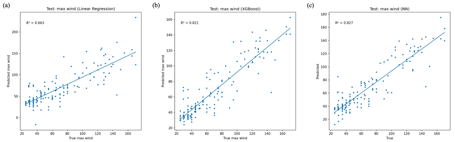
Model performance for peak maximum sustained wind was evaluated on the test set using the coefficient of determination (R²), root mean square error (RMSE), and mean absolute error (MAE). Results are summarized in Table 1. Both XGBoost and 3-layer NN significantly improves the prediction accuracy of the linear baseline, reducing the RMSE by over 25%. The RMSE of the neural network is slightly lower than that of XGBoost, indicating marginal gains in high-intensity domains where nonlinear relationships dominate.

3.2. Minimum central pressure

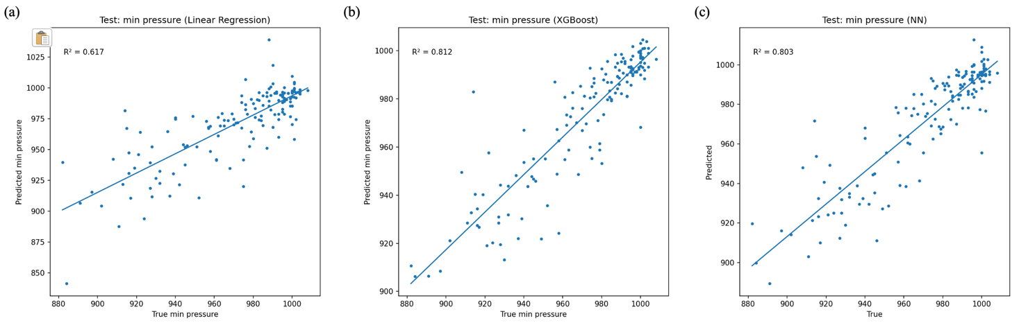
An analogous evaluation was performed for peak minimum central pressure. Model performance metrics are reported in Table 2. A trend similar to wind speed predictions can also be observed here, where XGBoost and 3-layer NN largely improve the predictions from the linear regression baseline. Relative to linear regression, XGBoost reduces RMSE by 29.85%, representing a significant enhancement in predictive performance. Unlike the wind speed task, the neural network does not outperform XGBoost, suggesting that the latter’s tree-based structure captures the nonlinear dependencies in pressure data more effectively.

3.3. Error structure and stratified performance

To investigate the performance of the three models across different Typhoon subgroups, stratified performance is independently calculated based on calendar month of the peak, latitude of the peak, and max intensity. The results are shown in Table 3.

The analysis reveals three consistent patterns. First, both XGBoost and the neural network systematically outperform the linear baseline across most partitions. They reduce stratified RMSE in the month groups, in latitude bands, and for every intensity class. The improvement is most pronounced for the strongest storms (TY and Super-TY), where nonlinear methods lower errors substantially. This is probably due to the fact that the driven factor of the stronger storms are complicated and thus the relationship between important predictors and peak intensity could not be adequately captured by linear regressions.

Second, error magnitude increases with intensity. Weak and moderate systems (TD/TS) show relatively low stratified RMSE, but errors rise for major typhoons and especially super typhoons. The most likely causes are (1) rarity of extreme cases in the training data, (2) larger intrinsic variability in rapid intensification events, and (3) potentially missing environmental covariates (e.g. vertical shear, SST) that modulate extreme intensification.

Last, spatial and seasonal structure is present. Mid-latitude bands and certain months show different error levels, suggesting geographic and seasonal modulation of predictability. However, conclusions based on month are affected by sample size limitations in some bins and missing month metadata for many records.

3.4. Feature contribution and sensitivity

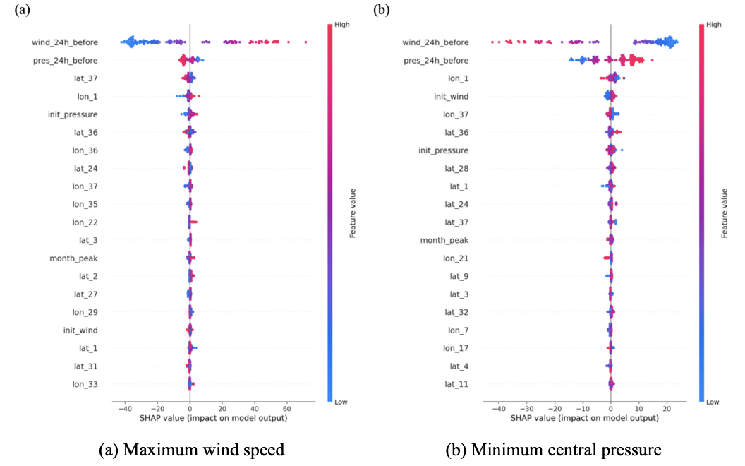
Unlike computer vision methods that learn from data including satellite images, our approach relies on tabular features composed of tracks and conventional meteorological quantities. For XGBoost, the top five factors ranked by gain for the maximum wind speed target are: wind speed 24 hours prior, pressure 24 hours prior, latitude 24 hours prior, initial longitude, and initial pressure; for the minimum pressure target, the top five factors are: wind speed 24 hours prior, pressure 24 hours prior, initial longitude, initial wind speed, and longitude 24 hours prior. The direction of the linear regression coefficients generally aligns with the XGBoost significance, further supporting the dominant role of wind/pressure 24 hours prior peak and track endpoint in intensity prediction. Figure 3 provides a summary of the feature effects of XGBoost models.

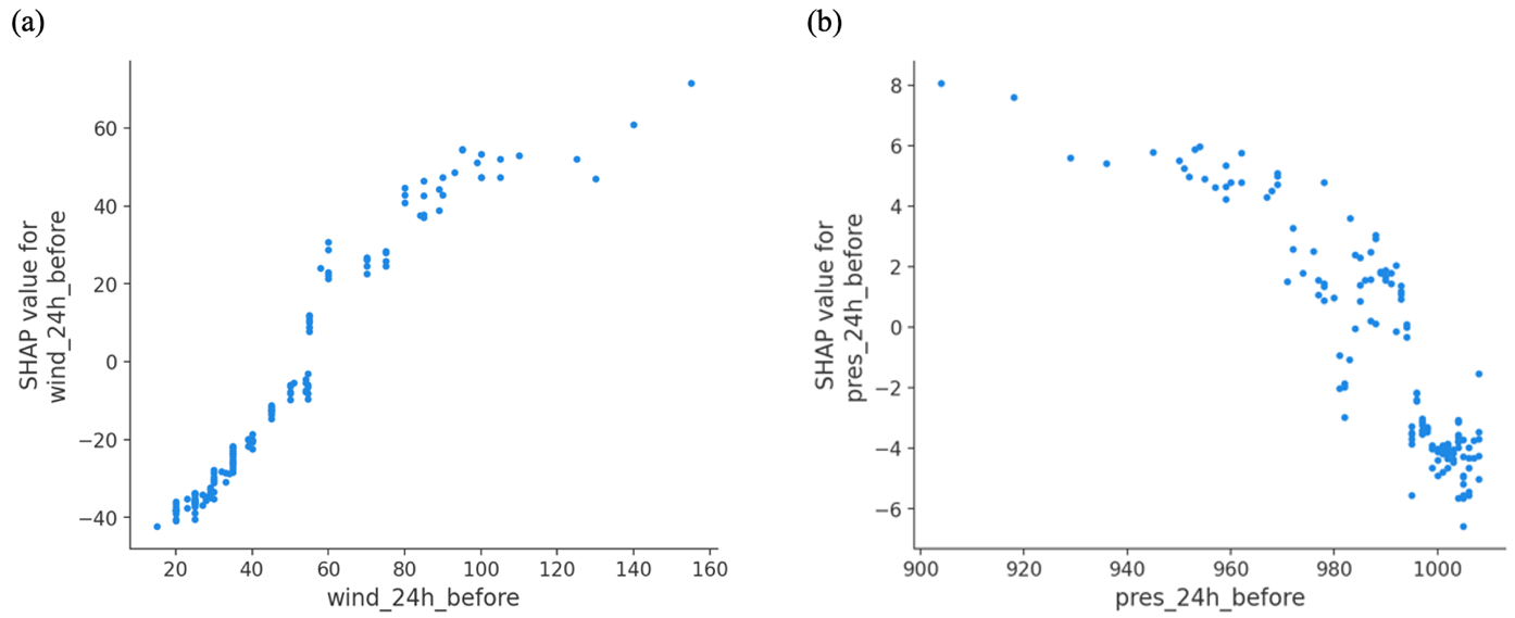
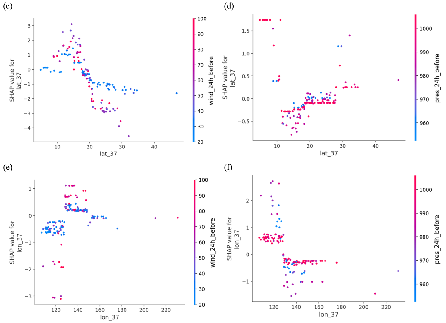
The partial-dependence (SHAP dependence) plots (Figure 4) for the scalar covariates highlight strong, monotone relationships with peak-wind prediction. Prior intensity is the dominant driver: wind_24h_before shows a close-to-linear, positive association with SHAP values across its range (Figure 4(a)). In contrast, pres_24h_before exhibits a complementary, monotone negative association (Figure 4(b)), higher pressures correspond to lower SHAP values, i.e., decreased predicted peak wind. The curvature at the low-pressure end hints that once central pressure drops below ~970–975 hPa, additional pressure falls carry smaller marginal gains in predicted peak wind in the model.

Spatial predictors contribute primarily through interactions with recent intensity. For latitude (Figure 4(c) and 4(d)), higher latitudes reduce predicted peak wind overall, but the gradient depends on recent conditions. When wind_24h_before is high, SHAP values decline more steeply with increasing latitude, consistent with stronger storms being more sensitive to poleward movement such as increased shear and cooler sea surface temperatures (SST). When prior wind is low, the decline is gentler and more stable, indicating a weaker penalization for latitude. Coloring by pres_24h_before shows a similar interaction from the opposite angle: less developed storms with higher pressure dampens the magnitude of the latitude penalty. Longitude effects (Figure 4(e) and 4(f)), are weaker on average but appear regime-dependent, with recognizable clusters around 120–150°E: storms situated westward are closer to land and marginal seas, and tend to receive slightly more negative SHAP contributions, particularly when prior wind is low or pressure is high, whereas eastward, open-ocean locations are associated with modestly positive contributions, especially for already strong systems. Together, these patterns indicate that spatial terms matter primarily as modulators—they amplify or attenuate the influence of recent intensity, rather than acting as strong main-effect predictors on their own.

3.5. Summary

On the post-2020 test set, nonlinear models markedly outperformed the linear baseline for both targets. For peak wind, XGBoost and a 3-layer NN cut RMSE from 22.77 kt to 16.60–16.29 kt and raised R² from 0.66 to 0.82–0.83, with the NN delivering a small edge at the highest intensities. For minimum pressure, XGBoost performed best (R²=0.81; RMSE 13.23 hPa), reducing error by ~30% versus linear regression. Stratified analyses discovered robust patterns across months, latitude bands, and intensity classes and error increases with intensity and changes with seasonal and geographic subgroups, though some month bins are sample-limited. Feature attribution identified 24-h prior wind and pressure as dominant predictors, with endpoint latitude/longitude contributing mainly through interactions. Overall, track-based models using a few readily available covariates provide accurate 24-h peak-intensity guidance, with tree ensembles offering the best accuracy–robustness trade-off.

4. Discussion

Using a parsimonious feature set, we obtain reliable 24-h peak-intensity forecasts. Relative to the linear baseline, XGBoost’s lower errors confirm that nonlinear interactions in track–intensity dynamics carry substantial signal even without rich environmental inputs. The learned relations are physically plausible: recent track geometry encodes synoptic setup (steering, curvature, land approach), T−24 h intensity provides persistence, and month supplies seasonal priors. Residual errors concentrate in extreme and transition regimes (e.g., eyewall replacement, land-interaction), where track-only features underrepresent the governing physics. These findings position the track-based model as a fast, data-light prior that can be strengthened by fusing compact environmental or satellite features in future work.

4.1. Practical implications

Relative to image-based or ML–NWP hybrids, our approach is data-parsimonious and fast, trading some absolute accuracy for replicability and transparency. Prior work that fuses satellite texture and environmental fields can achieve lower errors, but at the cost of heavy data pipelines. We show that a track-only, fixed pre-peak horizon baseline—evaluated at the storm level—already delivers useful skill and offers a sturdy benchmark onto which richer predictors can be layered.

Operationally, this makes a low-latency prior for agencies facing delays in satellite/reanalysis ingestion: inputs come from widely disseminated best-track feeds, so deployment is straightforward. Mapping continuous outputs to actionable tiers (e.g., TS/TY) can streamline communication, provided thresholds are locally calibrated. The design remains portable and interpretable—a transparent temporal split (pre-2020 train vs. post-2020 test, 151 storms) approximates out-of-sample generalization, and the small, physics-motivated feature set yields coefficients and importances that align with persistence, recent motion, and seasonal context.

4.2. Limitations

First, label heterogeneity arises from pairing JMA/Tokyo tracks with JTWC intensities; differences in averaging periods, quality control, and peak-time conventions likely introduce nontrivial noise despite unit harmonization. Second, the absence of environmental covariates (e.g., SST, vertical wind shear, ocean heat content) and satellite texture—likely caps performance, particularly for rapidly evolving or extreme regimes.

Third, the fixed horizon and sequence length (37 pre-peak points at T–24 h) standardizes inputs but may penalize short-lived storms and underrepresent earlier lifecycle variability. Finally, temporal drift and class imbalance remain concerns: post-2020 changes in observing/reporting practices and the scarcity of TY/Super-TY cases can affect transportability and calibration, underscoring the value of era-aware validation and uncertainty-aware evaluation in the future.

4.3. Future work

Future work improving on this framework should consider adding compact environmental summaries (e.g., shear and SST at T−24 h and along-track means), and optionally a lightweight satellite channel to inject structural information with minimal pipeline cost, move from point estimates to quantile/interval predictions so that end-users receive calibrated ranges, replace manual waypoint selection with sequence models (e.g., 1D CNN/transformer over the track) to learn temporal patterns directly while keeping inputs tabular. Stress tests such as evaluating on data from different regions can help reduce overfit and assess transportability and the need for region-specific recalibration. It will also be valuable to quantify the marginal value of each feature group and ensure performance is not systematically worse for near-landfall peaks or short-track storms through ablations and fairness checks.

5. Conclusion

This study demonstrates that a parsimonious, track-centric approach can provide accurate 24-hour forecasts of tropical-cyclone peak intensity, with nonlinear models substantially outperforming a linear baseline for both maximum wind and minimum pressure. By standardizing pre-peak histories and using readily available best-track covariates, the framework delivers skill that is portable, fast to deploy, and interpretable—qualities that make it a useful low-latency prior when environmental or satellite inputs are delayed or unavailable. Stratified analyses highlight consistent gains across seasons, latitude bands, and intensity classes, while also revealing larger errors for the most extreme systems, underscoring the limits of track-only information. Key constraints include label heterogeneity, omission of environmental and satellite predictors, and a fixed pre-peak horizon. Future extensions that fuse compact environmental fields or satellite features, incorporate uncertainty quantification, and explore sequence encoders or cross-basin validation are likely to improve performance and operational reliability, positioning track-based learning as a practical complement to more data-intensive forecasting systems.

Acknowledgement

I gratefully acknowledge Yupeng Chen for his insightful guidance and constructive feedback, which were invaluable to the completion of this paper.

References

[1]. A. M. F. Lagmay et al., “Devastating storm surges of Typhoon Haiyan, ” Int. J. Disaster Risk Reduct., vol. 11, pp. 1–12, Mar. 2015, doi: 10.1016/j.ijdrr.2014.10.006.
[2]. “Typhoon Yagi killed 318 people, damage reaches $3.3 billion, ” vietnamnews.vn. Accessed: Oct. 05, 2025. [Online]. Available: https: //vietnamnews.vn/society/1663938/typhoon-yagi-killed-318-people-damage-reaches-3-3-billion.html
[3]. X. Bi, J. Liu, and Y. Duan, “Review of Artificial Intelligence Application in Typhoon Forecasting, ” Trop. Cyclone Res. Rev., p. S2225603225000311, Jul. 2025, doi: 10.1016/j.tcrr.2025.07.005.
[4]. R. Chen, W. Zhang, and X. Wang, “Machine Learning in Tropical Cyclone Forecast Modeling: A Review, ” Atmosphere, vol. 11, no. 7, p. 676, Jun. 2020, doi: 10.3390/atmos11070676.
[5]. H. Xu, Y. Zhao, Z. Dajun, Y. Duan, and X. Xu, “Exploring the typhoon intensity forecasting through integrating AI weather forecasting with regional numerical weather model, ” Npj Clim. Atmospheric Sci., vol. 8, no. 1, p. 38, Feb. 2025, doi: 10.1038/s41612-025-00926-z.
[6]. A. S. Albahri et al., “A systematic review of trustworthy artificial intelligence applications in natural disasters, ” Comput. Electr. Eng., vol. 118, p. 109409, Sep. 2024, doi: 10.1016/j.compeleceng.2024.109409.
[7]. A. Mosavi, P. Ozturk, and K. Chau, “Flood Prediction Using Machine Learning Models: Literature Review, ” Water, vol. 10, no. 11, p. 1536, Oct. 2018, doi: 10.3390/w10111536.
[8]. K. M. Asim, A. Idris, T. Iqbal, and F. Martínez-Álvarez, “Earthquake prediction model using support vector regressor and hybrid neural networks, ” PLOS ONE, vol. 13, no. 7, p. e0199004, Jul. 2018, doi: 10.1371/journal.pone.0199004.
[9]. J. Buch, A. P. Williams, C. S. Juang, W. D. Hansen, and P. Gentine, “SMLFire1.0: a stochastic machine learning (SML) model for wildfire activity in the western United States, ” Geosci. Model Dev., vol. 16, no. 12, pp. 3407–3433, Jun. 2023, doi: 10.5194/gmd-16-3407-2023.
[10]. L. Jin, C. Yao, and X.-Y. Huang, “A Nonlinear Artificial Intelligence Ensemble Prediction Model for Typhoon Intensity, ” Mon. Weather Rev., vol. 136, no. 12, pp. 4541–4554, Dec. 2008, doi: 10.1175/2008MWR2269.1.
[11]. F. Meng, Y. Yao, Z. Wang, S. Peng, D. Xu, and T. Song, “Probabilistic forecasting of tropical cyclones intensity using machine learning model, ” Environ. Res. Lett., vol. 18, no. 4, p. 044042, Apr. 2023, doi: 10.1088/1748-9326/acc8eb.
[12]. H. Liu et al., “A Hybrid Machine Learning/Physics‐Based Modeling Framework for 2‐Week Extended Prediction of Tropical Cyclones, ” J. Geophys. Res. Mach. Learn. Comput., vol. 1, no. 3, p. e2024JH000207, Sep. 2024, doi: 10.1029/2024JH000207.
[13]. X.-Y. Xu, M. Shao, P.-L. Chen, and Q.-G. Wang, “Tropical Cyclone Intensity Prediction Using Deep Convolutional Neural Network, ” Atmosphere, vol. 13, no. 5, p. 783, May 2022, doi: 10.3390/atmos13050783.
Cite this article
Yu,Y. (2025). Track-Centric Machine Learning for 24-Hour Peak-Intensity Forecasting of Western North Pacific Typhoons. Applied and Computational Engineering,196,14-23.
Data availability
The datasets used and/or analyzed during the current study will be available from the authors upon reasonable request.
Disclaimer/Publisher's Note
The statements, opinions and data contained in all publications are solely those of the individual author(s) and contributor(s) and not of EWA Publishing and/or the editor(s). EWA Publishing and/or the editor(s) disclaim responsibility for any injury to people or property resulting from any ideas, methods, instructions or products referred to in the content.
About volume
Volume title: Proceedings of CONF-MLA 2025 Symposium: Intelligent Systems and Automation: AI Models, IoT, and Robotic Algorithms
© 2024 by the author(s). Licensee EWA Publishing, Oxford, UK. This article is an open access article distributed under the terms and
conditions of the Creative Commons Attribution (CC BY) license. Authors who
publish this series agree to the following terms:
1. Authors retain copyright and grant the series right of first publication with the work simultaneously licensed under a Creative Commons
Attribution License that allows others to share the work with an acknowledgment of the work's authorship and initial publication in this
series.
2. Authors are able to enter into separate, additional contractual arrangements for the non-exclusive distribution of the series's published
version of the work (e.g., post it to an institutional repository or publish it in a book), with an acknowledgment of its initial
publication in this series.
3. Authors are permitted and encouraged to post their work online (e.g., in institutional repositories or on their website) prior to and
during the submission process, as it can lead to productive exchanges, as well as earlier and greater citation of published work (See
Open access policy for details).