1. Introduction

Currently, addressing climate change and ensuring energy security have become core global issues. Against this backdrop, clean and renewable energy, represented by wind energy, is developing at an unprecedented rate, driving profound changes in the global energy system [1]. Wind power generation has become the main force in renewable energy generation due to its abundant resources, mature technology, and environmental friendliness. However, large-scale wind power grid integration also poses severe challenges to the planning, scheduling, and operation of power systems [2,3]. Wind, as a manifestation of atmospheric flow, is affected by a variety of complex factors such as topography, climate, temperature, and air pressure, resulting in strong randomness, volatility, and intermittency in wind speed and direction. This uncertainty is directly transmitted to the output power of wind turbines, making wind power an unstable power source and posing a potential threat to grid frequency regulation, voltage stability, backup capacity configuration, and the fairness of power market transactions [4,5].

To meet these challenges and achieve efficient and reliable utilization of wind energy resources, it is particularly important to accurately predict wind power. According to the prediction time scale, wind power prediction can be divided into four categories: long-term, medium-term, short-term and ultra-short-term [6]. Among them, medium- and long-term predictions (especially predictions for the next 24–72 hours) are of great practical significance and are directly related to the power system's power generation plan formulation, grid operation mode arrangement, ancillary service market decision-making and electricity spot market quotation strategy [7]. An accurate long-term prediction system can effectively reduce the system backup cost caused by wind power uncertainty, reduce wind curtailment and power rationing, and improve the safety and economy of grid operation [8].

Traditional wind power prediction methods are mainly divided into physical methods and statistical methods. The physical method uses numerical weather forecast data and geographical features to convert meteorological data into wind speed and direction at the turbine hub height, and then estimates the power output through the power-wind speed curve [8,9]. This method does not rely on a large amount of historical data and is suitable for new wind farms. However, its prediction accuracy is heavily dependent on the quality of NWP data, and the modeling is complex, time-consuming and costly [10].

With the advancement of artificial intelligence, neural networks such as multilayer perceptron’s, convolutional neural networks, and temporal convolutional networks have been introduced to the field of wind power forecasting, driving technological innovation in this area. In particular, RNN-based models (such as LSTM and GRU) have attracted considerable attention due to their exceptional ability to capture temporal dependencies. In recent years, the Transformer, leveraging its self-attention mechanism to capture global temporal dependencies, has become a key tool for time series forecasting. However, existing Transformer-based models still face the challenge of limited context length when processing long-term wind power series. Unlike Transformers in natural language and vision tasks, which can process thousands to millions of tokens, time series Transformers typically operate within a limited context of only a few hundred-time steps, resulting in insufficient learning of global trends and difficulty in effectively addressing non-stationarity. Furthermore, the importance of explicitly capturing both intra- and inter-channel dependencies in multivariate forecasting has become increasingly prominent, making it imperative to expand the context length to encompass more relevant time series.

In this following, this paper introduces a blocking operation to divide the original sequence into local segments to expand contextual information and improve the information integrity of the Transformer. To address the noise problem in the training data, the VMD module is used to compress the signal energy distribution in the frequency domain to reduce the impact of noise. The Time Attention mechanism is further proposed. This mechanism is designed for multidimensional time series, has position-aware capabilities, can simultaneously model intra-sequence and inter-sequence dependencies, and maintain the causality and scalability of the Transformer.

2. Time attention transformer prediction method

2.1. Prediction method framework

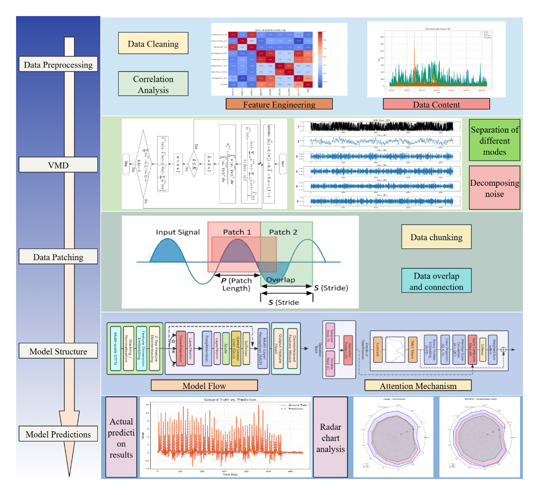
The overall framework proposed in this paper first performs preprocessing operations such as missing value filling and standardization on historical data containing complex periodicity and high volatility. It then adopts a "decomposition-forecasting" strategy, using VMD to decompose the original time series into multiple intrinsic mode components that are easier to model. After block partitioning and filtering, the components are input into an improved Transformer model for training. Finally, the accuracy and effectiveness of the forecasting framework are fully verified by visually comparing the forecast results with the true values and quantitatively evaluating them using metrics such as root mean square error, mean absolute error, and mean square error. The specific process is shown in Figure 1.

2.2. VMD signal decomposition

Variational mode decomposition (VMD), a non-recursive signal decomposition method with a solid mathematical foundation, has garnered widespread attention in recent years. VMD frames the signal decomposition process as a constrained variational problem, aiming to find a set of modal components with specific center frequencies whose sum of bandwidths minimizes while accurately reconstructing the original signal. Compared to empirical mode decomposition (EMD) and its variants, VMD performs better in suppressing modal aliasing and improving robustness. This paper uses VMD to decompose long-term wind power data. The detailed process is shown in Figure 2.

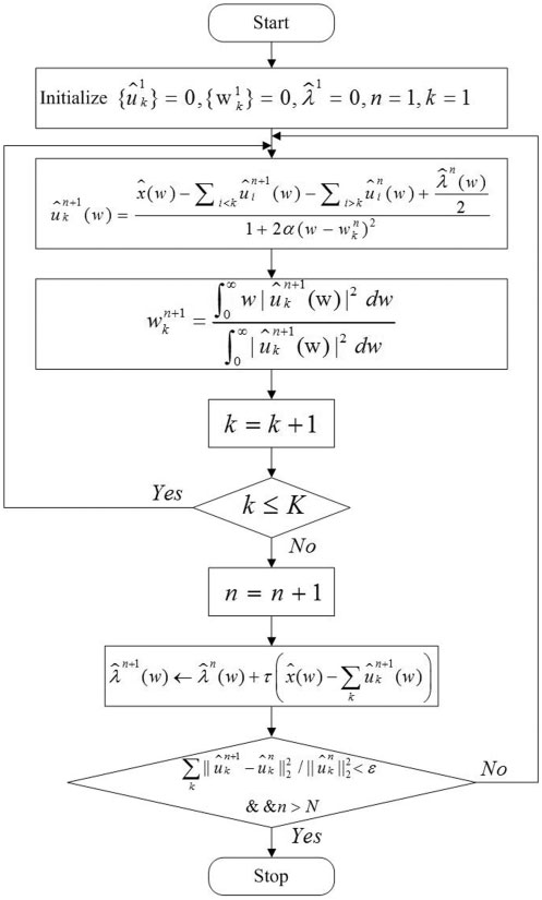
The essence of VMD is an iterative optimization process that aims to decompose an original signal into a preset number (K) of intrinsic mode functions (IMFs) with specific center frequencies. Its core iterative update process mainly includes the following three formulas:

In the (n+1)th iteration, the frequency domain representation of the kth modal component is updated according to the following formula. This update is implemented in the frequency domain using a Wiener filter to extract the components around the center frequency from the current residual signal. The specific formula is as follows:

$$ {\widehat{u}}_k^{n+1}\left(\omega \right)=\frac{\widehat{x}\left(\omega \right)-\sum _{i<k}{\widehat{u}}_i^{n+1}\left(\omega \right)-\sum _{i>k}{\widehat{u}}_i^n\left(\omega \right)+\frac{{\widehat{\lambda }}^n\left(\omega \right)}{2}}{1+2\alpha {\left(\omega -{\omega }_k^n\right)}^2}$$(1)

Among them, refers to the  $$ {\widehat{\mathrm{u}}}_{\mathrm{k}}^{\mathrm{n}+1}\left(\mathrm{\omega }\right)$$ kth mode obtained after this iterative update;

 $$ \widehat{\mathrm{x}}\left(\mathrm{\omega }\right)$$ Refers to the Fourier transform of the original signal;

 $$ \sum _{\mathrm{i}<\mathrm{k}}{\widehat{\mathrm{u}}}_{\mathrm{i}}^{\mathrm{n}+1}\left(\mathrm{\omega }\right)$$ Refers to other modalities that have been updated in this iteration;

 $$ \sum _{\mathrm{i}>\mathrm{k}}{\widehat{\mathrm{u}}}_{\mathrm{i}}^{\mathrm{n}}\left(\mathrm{\omega }\right)$$ Refers to other modes obtained in the previous iteration;

 $$ {\widehat{\mathrm{\lambda }}}^{\mathrm{n}}\left(\mathrm{\omega }\right)$$ Refers to the Lagrange multiplier of the previous iteration, which is used to constrain the sum of all modes to be equal to the original signal;

 $$ \mathrm{\alpha }$$ A quadratic penalty factor, which controls the strictness of the constraint;

 $$ {\mathrm{\omega }}_{\mathrm{k}}^{\mathrm{n}}$$ kth mode obtained in the previous iteration.

After updating the modal component, its center frequency needs to be recalculated to locate the place where the modal energy is most concentrated. This process is equivalent to calculating the center of gravity of the modal power spectrum. The specific formula is as follows:

$$ {\omega }_k^{n+1}=\frac{{\int }_0^{\mathrm{\infty }}\omega {\left|{\widehat{u}}_k^{n+1}\left(\omega \right)\right|}^{2}d\omega }{{\int }_0^{\mathrm{\infty }}{\left|{\widehat{u}}_k^{n+1}\left(\omega \right)\right|}^{2}d\omega }$$(2)

This formula calculates the center of the power spectrum of the updated mode.

all K modes and their center frequencies are updated, the Lagrange multipliers need to be updated to better enforce the constraint that the sum of all modes is equal to the original signal in the next iteration.

$$ {\widehat{\lambda }}^{n+1}\left(\omega \right)={\widehat{\lambda }}^n\left(\omega \right)+\tau \left(\widehat{x}\left(\omega \right)-\sum _k{\widehat{u}}_k^{n+1}\left(\omega \right)\right)$$(3)

Among them,  $$ \mathrm{\tau }$$ : dual ascent step size (or called update parameter), which affects the convergence speed;

 $$ \widehat{\mathrm{x}}\left(\mathrm{\omega }\right)-\sum _{\mathrm{k}}{\widehat{\mathrm{u}}}_{\mathrm{k}}^{\mathrm{n}+1}\left(\mathrm{\omega }\right)$$ : This is the residual between the sum of all current modes and the original signal (i.e., reconstruction error). The purpose of the update is to reduce this residual in the next iteration.

2.3. Time attention transformer

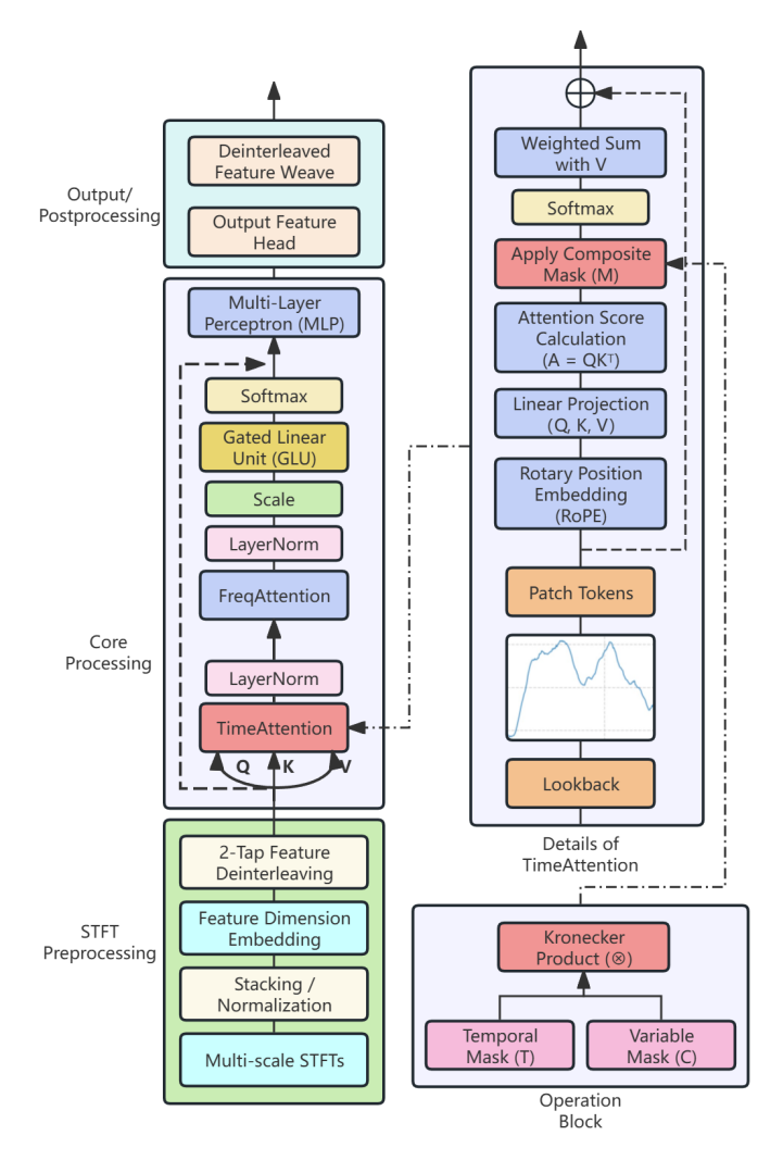
After segmenting wind power information, we constructed a causal model architecture based on a decoder-only Transformer to achieve unified prediction of heterogeneous time series tasks. The core of this architecture is to abandon the traditional global prediction paradigm and instead generalize the multi-dimensional time series prediction problem into a long-context next prediction task.

At the input representation layer of the model, after the original time series is tokenized into blocks, each token is first mapped to a high-dimensional feature space through an independent embedding matrix. This process can be expressed as:

$h_i^0=W_e{x}_i$(4)

To enable the model to perceive multidimensional data structures, we further introduce composite positional encoding: in the time dimension, rotated position embedding is used to inject temporal information; in the variable dimension, two learnable scalar parameters are used to distinguish between endogenous and exogenous information sources, thereby ensuring equivalence of the model's permutation order for variable input. The processed token representation sequence is then fed into a core network consisting of L identical stacked blocks for deep feature extraction. Each block contains a standard feedforward network and a TimeAttention mechanism, both connected by residual connections and layer normalization.

The key to TimeAttention lies in precisely controlling the flow of information through a hierarchical mask. This mask is generated by a Kronecker product (⊗) between a variable dependency mask (C) that defines the dependencies between variables and a temporal causal mask (T) that ensures temporal causality. This mask is combined with the original attention score matrix that includes position information to form the final attention calculation formula:

$$ TimeAttention\left(H\right)=\mathrm{ }Softmax\left(\frac{Mask\left(\mathcal{C}\otimes \mathcal{T}\right)+\mathcal{A}}{\sqrt{d_k}}\right)H{W}_v$$(5)

After L layers of processing, the model maps the final feature representation back to the prediction space through a token-level linear projection layer, generates a predicted value for the next token for each input position, and finally optimizes the model by minimizing the mean squared error between all predicted tokens and the true value. The internal specific process is shown in Figure 4:

3. Numerical results

3.1. Dataset preprocessing

To demonstrate the versatility of the model, this study used two different types of datasets for training and validation.

Dataset 1 is a univariate dataset with high temporal resolution. It accurately records the continuous wind power output within a specific region at a sampling interval of 15 minutes. The data is derived from actual grid operation records of four German transmission system operators, comprising one year's worth of data from each operator. This dataset is currently publicly available on Kaggle. The core characteristic of this dataset lies in its univariate nature: all observations collectively describe the dynamic evolution of a single physical quantity, wind power, over time. This time series typifies the inherent multi-scale periodicity of wind power generation, as well as the high degree of randomness and volatility caused by wind speed uncertainty.

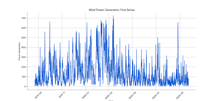
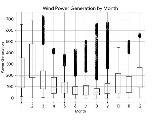
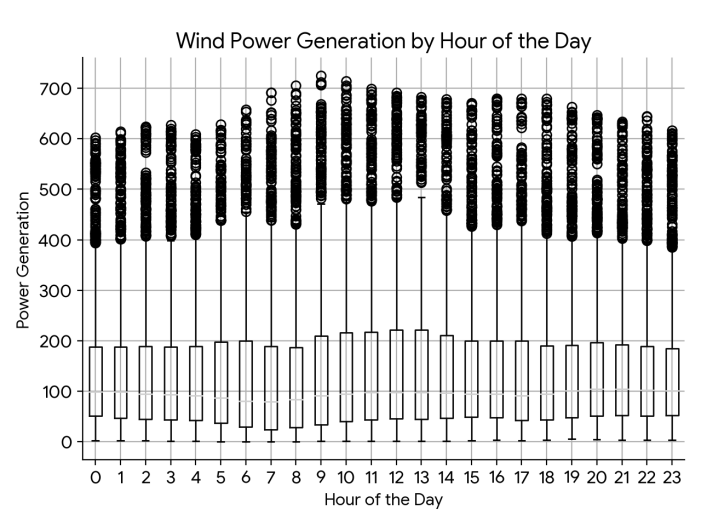
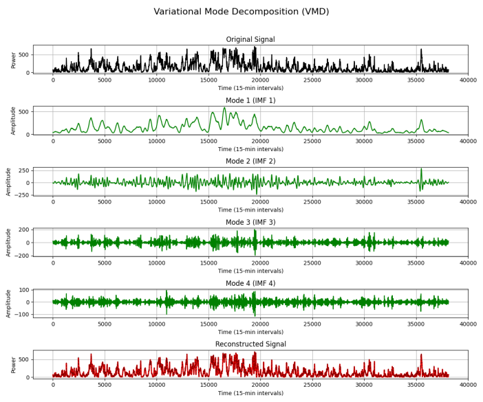
Figure 5 shows that the time series exhibits significant nonstationarity, with strong random fluctuations and clear periodic patterns. Figures 6 and 7 further confirm this, showing that the series can be clearly decomposed into three components: trend, seasonality, and residual. The trend term reveals the long-term variation of the data over the entire observation period, while the seasonal term reveals highly regular periodic patterns on a daily or weekly basis, consistent with the natural intra-day and seasonal variations in wind energy resources. The residual term represents the random noise component in the data. Figure 6 shows that the autocorrelation coefficient decays slowly with increasing lag order, exhibiting a significant tailing phenomenon, a typical characteristic of strong trend or seasonality in nonstationary time series. Furthermore, Figure 7 demonstrates rapid truncation. After lag one, the partial autocorrelation coefficient quickly falls within the confidence interval, indicating that the power value at the current moment is highly dependent on the value at the immediately preceding moment. Therefore, when constructing a prediction model for dataset 1, these complex dynamic characteristics must be fully considered and properly handled, such as through differencing, seasonal decomposition, or the use of algorithms that can directly model these characteristics to ensure the accuracy of the prediction.

Dataset 2 is a multivariate dataset derived from time series data from wind turbine sites at four different locations. This dataset is currently publicly available on Kaggle. This dataset details key meteorological indicators that influence wind power generation and the actual power output of the turbines. Data from each site include multiple physical quantities measured at different altitudes. Core indicators include temperature, relative humidity, dew point, and wind speed, wind gusts, and wind direction, which are crucial for power prediction. The target predictor variable is power, with standardized units. The data has an hourly granularity and covers a continuous observation period starting in early 2017. After integrating data from all four sites, the dataset contains a large number of continuous observation time steps, providing a rich data sample for training deep learning models. To construct a high-quality training set suitable for model use, we performed necessary preprocessing on the raw data and conducted correlation analysis on the various data points in the dataset. The results are shown in the figure below:

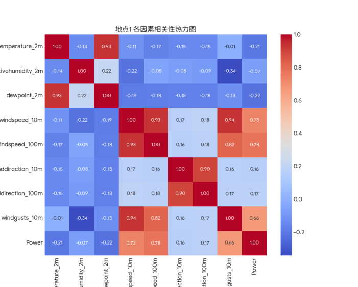
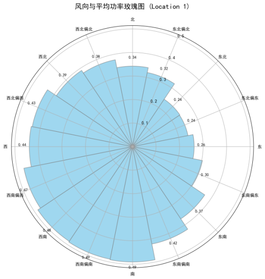
To build an efficient and relevant prediction model, we first analyzed the correlation between various meteorological features and the target variable, power generation, as shown in the feature correlation heat map. This analysis revealed a strong positive correlation between wind speed and power generation, making it the most significant driver of power output. In contrast, other meteorological variables such as temperature and air pressure also showed some correlation, but their impact was far less significant than that of wind speed. Based on this finding, this experiment focused on these highly correlated variables and constructed an input feature set to reduce model complexity and mitigate noise introduced by irrelevant variables.

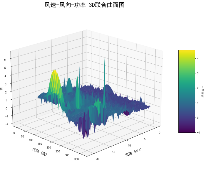
Figure 10 reveals its inherent high volatility and intermittency, with power values fluctuating dramatically over short periods of time. A 3D joint analysis of the key input features, wind speed and generated power, further intuitively confirms the strong dependency between the two. Their distribution exhibits the typical characteristics of a wind turbine power curve: between the cut-in wind speed and the rated wind speed, power rises sharply with increasing wind speed before leveling off. This clear nonlinear relationship is the key basis for building an accurate prediction model. A comprehensive analysis of the temporal variations and correlations of each input feature established a modeling strategy centered on wind speed, supplemented by other highly correlated meteorological factors. This strategy aims to fully utilize the most effective information to capture and predict the dynamic changes in wind power.

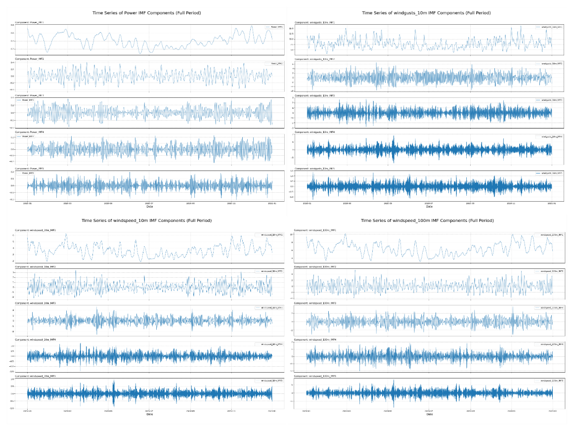
After the analysis is completed, as described above, the four most correlated data sets (Power, windspeed_100m, windspeed_10m, and windgusts_10m) are selected and VMD decomposition is performed on the data into 20 modal data. This ultimately forms a new dataset, which provides a solid foundation for subsequent model learning and evaluation on multivariate and long time series dependencies.

3.2. Evaluation method

To objectively measure and compare the performance of different forecasting models, a set of standardized evaluation metrics is required. These metrics quantify the deviation between the predicted and true values from different perspectives and are important tools for verifying model effectiveness. In wind power forecasting, the most commonly used metrics include mean absolute error (MAE), root mean square error (RMSE), and mean absolute percentage error (MAPE). MAE, by calculating the average of the absolute values of the forecast errors, intuitively reflects the average deviation of the forecast results, using the same units as the original data.

$MSE=\frac{1}{n}{\sum }_{i=1}^n({\widehat{y}}_i-y_i{)}^2$(6)

$$ MAE=\frac{1}{n}\sum _{i=1}^n\left|{\widehat{y}}_i-y_i\right|$$(7)

$RMSE=\sqrt{\frac{1}{n}{\mathrm{\Sigma }}_{i=1}^n({\widehat{y}}_i-y_i{)}^2}$(8)

MAE is the average of the absolute errors of all individual observations. It directly reflects the average size of the model's prediction errors. Unlike MAE, MSE amplifies the impact of larger errors on the overall error by squaring the errors. This means that MSE is very sensitive to outliers in the model's predictions. If the model exhibits significant deviations at certain points, the MSE value will increase significantly. RMSE is one of the most widely used regression model evaluation metrics. By taking the square root of the MSE, the units of the RMSE are restored to match those of the original data, thus resolving the issue of the MSE's difficulty in interpreting the numerical value. Like MSE, RMSE also places greater weight on larger prediction errors, making it equally sensitive to outliers. The RMSE value can be intuitively understood as the average "distance" or "deviation" between the model's predictions and the true values.

In summary, MAE provides a direct measure of the average error, while MSE and RMSE focus more on penalizing larger errors. In model evaluation, we usually refer to these three indicators simultaneously to comprehensively and objectively evaluate the predictive performance and stability of the model.

3.3. Results analysis

This section systematically presents and analyzes the results of various experiments, including main experimental comparisons with baseline models and ablation experiments to verify the effectiveness of each component of the model.

3.3.1. Comparative results

To comprehensively evaluate the effectiveness of the proposed model, we conducted a series of exhaustive experiments on two public datasets and compared its performance with 12 mainstream baseline models, including advanced attention-based models such as the Transformer, Informer, and Autoformer, as well as classic LSTM and MLP models. The experimental results were evaluated using mean squared error, mean absolute error, and root mean squared error. The results are shown in Table X.

Based on all experimental results, the model proposed in this paper shows the best performance under all test conditions, significantly surpassing all benchmark models. The specific results are shown in the figure below:

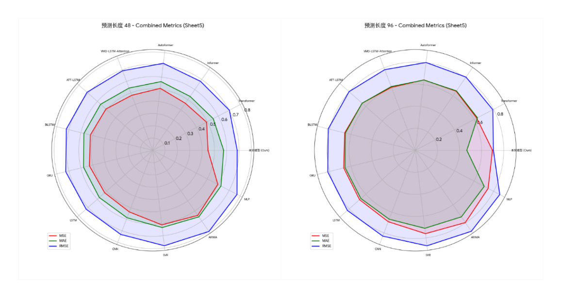
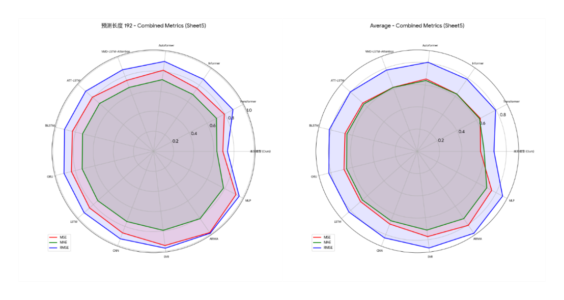
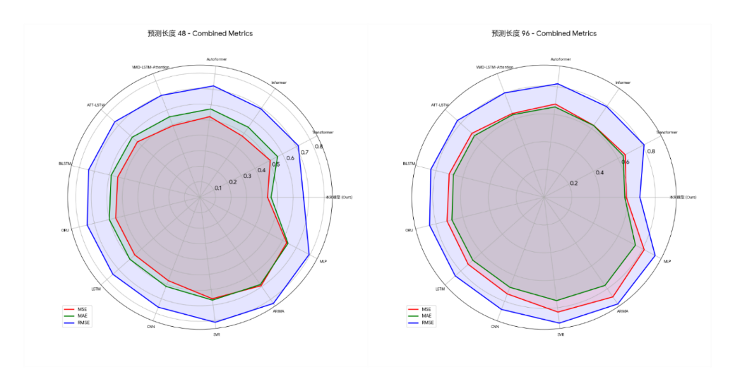
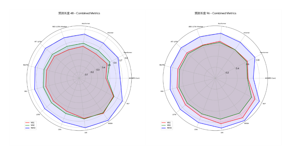
Across all datasets and prediction lengths tested, our model achieved the lowest or second-lowest error metrics. Taking the experimental data in Table 4 of "Dataset 1" as an example, the model achieved the best average mean squared error (MSE), mean absolute error (MAE), and root mean squared error (RMSE) across all prediction lengths, reaching 0.568, 0.601, and 0.689, respectively. Within specific prediction tasks, the model's strengths varied across scenarios: For short-term tasks with a prediction length of 48, it achieved the lowest mean squared error (MSE) of 0.448. Its advantage was most pronounced for the most challenging long-term tasks with a prediction length of 192, achieving the best MSE, MAE, and RMSE of 0.689, 0.630, and 0.735, respectively. For medium-term tasks with a prediction length of 96, although the VMD-LSTM-Attention model achieved the lowest MSE, our model achieved the best RMSE and MAE, demonstrating its superiority in controlling extreme errors.

Furthermore, the advantages of this model are not limited to specific scenarios, but are consistent across all evaluation dimensions. Whether it is short-term prediction or the more challenging long-term prediction, the model in this paper can maintain the lowest error rate. For example, in the long-term prediction task with a prediction length of 192 in "Dataset 2", the RMSE of this model is 0.728, which is significantly lower than all other comparison models, demonstrating its stability and robustness in long-term prediction tasks. By verifying on two datasets with different characteristics, the model in this paper always maintains a leading position, which strongly demonstrates its strong generalization ability and adaptability to long-term wind power data. From the average performance of the experiment, the average error value of the model in this paper is significantly lower than that of all baseline models, among which the closest Informer model has an average error of 0.672.

Multi-dimensional visualizations of the experimental results provide a comprehensive perspective for evaluating model performance. For all models, forecast errors systematically increase with increasing forecast length. This trend aligns with the fundamental principle of increasing uncertainty in time series forecasting, thereby validating the overall experimental framework. Within this framework, visualizations such as performance heatmaps and three-dimensional bar charts consistently demonstrate that the proposed model outperforms all baseline models. Specifically, the model achieves the lowest error across all twelve test scenarios, with its leading performance highlighted in the charts. This consistent performance across multiple scenarios demonstrates that the model's performance improvement is robust and consistent, not limited to specific evaluation criteria. These detailed and consistent visualizations demonstrate, from multiple perspectives, that the proposed model achieves superior forecast accuracy and robustness compared to the baselines.

3.3.2. Result analysis

To further verify the effectiveness and performance of the proposed wind power prediction model, this section provides a detailed analysis of the model's experimental results on a test set separated from the two datasets mentioned above. Typical prediction results are shown in Figures 18 and 19.

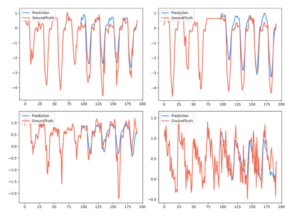
As can be clearly seen in Figure 18, the model demonstrates excellent univariate time series forecasting performance on a univariate wind power dataset. Driven solely by historical data, the model's forecast curves closely match the future true values, successfully reproducing future power trends with high fidelity across the three key dimensions of phase, amplitude, and waveform. This outstanding performance not only validates the model's strong generalization capabilities on a novel dataset but, more importantly, demonstrates its ability to uncover profound dynamic dependencies solely from the sequence itself. Even under complex operating conditions with weaker periodicity and greater randomness, the model maintains robust forecasting performance, demonstrating its strong robustness.

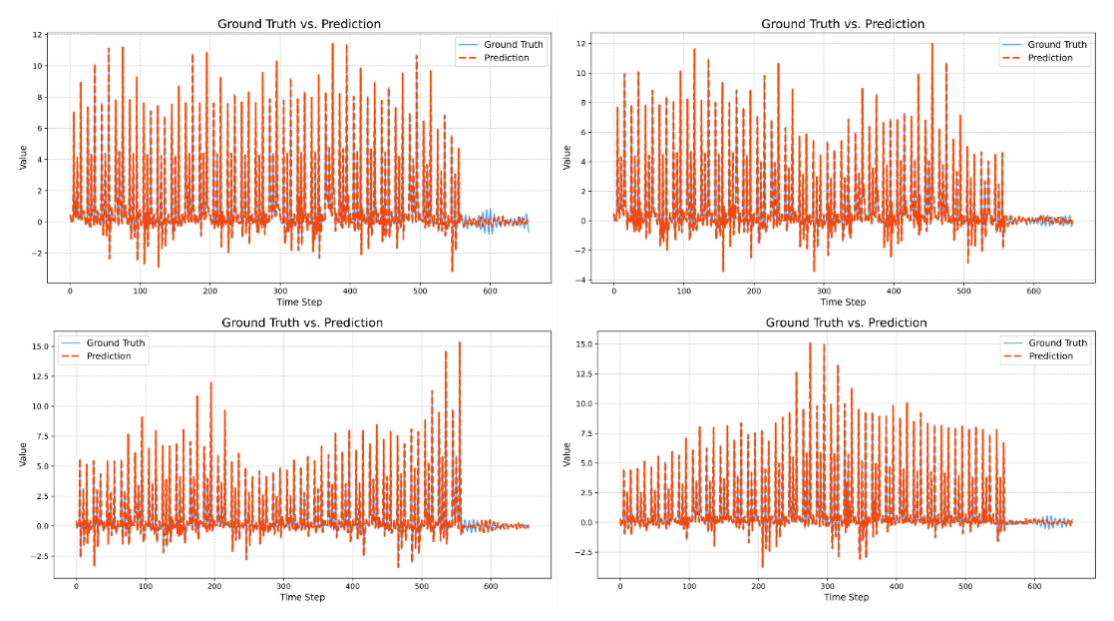
Figure 19 clearly shows that the power curves predicted by this model and the observed power curves for multivariate wind power data show a high degree of goodness of fit overall. The fluctuation trends, amplitudes, and phases of the two curves are largely consistent, intuitively demonstrating the proposed model's powerful nonlinear mapping capabilities and high-precision prediction performance. Even in regions where wind power exhibits significant fluctuations and strong randomness, the model still provides reliable predictions.

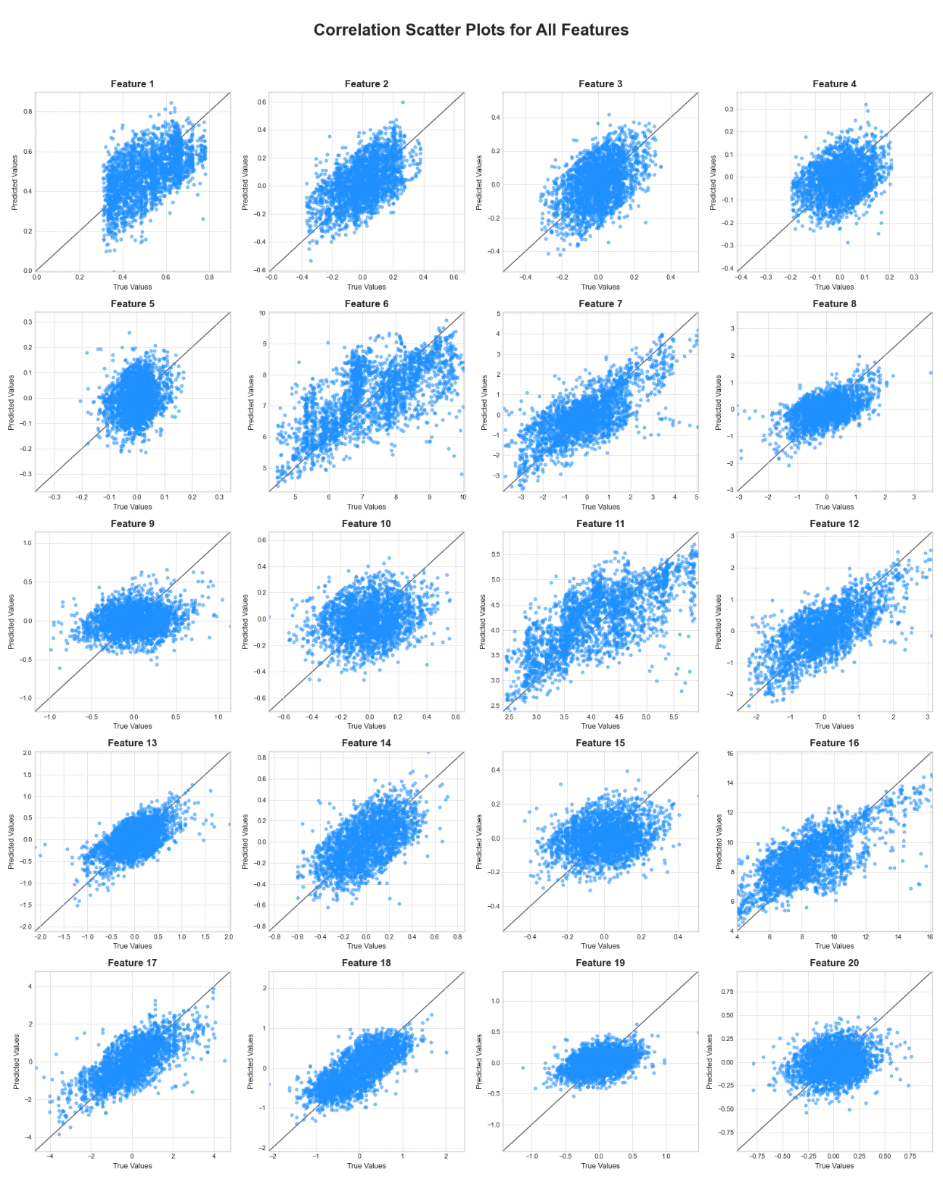
Figure 20 shows a scatter plot of the correlation between the predicted values and the true values for the 20 input features of the proposed model. In each subplot, the diagonal line represents an ideal, error-free, perfect prediction. Therefore, the distribution of the data point cloud can intuitively reflect the model's predictive performance for the corresponding feature. The more closely the point cloud is linearly distributed around the diagonal line, the higher the prediction accuracy; conversely, the more diffuse the point cloud is, the worse the prediction performance. A comprehensive analysis of all subplots reveals that the most striking conclusion is that this model is not a simple, homogeneous predictor, but rather a highly intelligent differential learning system. It accurately identifies the signal-to-noise ratio and regularity of different features and adjusts its prediction strategy accordingly, achieving high-fidelity reproduction for "predictable" features and providing valuable trend analysis for "highly random" features.

The above experimental results show that this model performs well in three key aspects in multivariate data:

Accurate trend tracking: The model's predictions quickly and accurately tracked the actual power values during rapid power increases, high-level plateaus, and rapid power decreases. This demonstrates that the model successfully learned the deep connection between the key external factors driving power changes and output power, rather than simply lagging behind and mimicking it.

Effectively learning cyclical patterns: The model effectively captures the cyclical patterns inherent in the wind power series. The peaks and troughs of the predicted curve coincide closely with the actual curve, accurately reproducing the fluctuations in wind power. This demonstrates that the model successfully exploits the inherent temporal dependencies of time series data, making its forecasts highly forward-looking.

Excellent adaptability to operating conditions: In the latter part of Figure 2.5-1, the wind farm's operating conditions change significantly, with power output switching from a highly fluctuating state to a sustained low power output. At this critical transition point, the model demonstrates exceptional adaptability. It keenly identifies this fundamental shift in system conditions and rapidly adjusts the predicted output to a low range consistent with actual conditions, maintaining a consistently low prediction error. This performance demonstrates not only the model's excellent predictive capabilities for typical fluctuations but also its high robustness and environmental adaptability to sudden changes in system operating modes.

In summary, a systematic analysis of the experimental results demonstrates that the proposed wind power prediction model excels in overall performance, trend tracking, periodicity capture, and adaptability to operating conditions. The high sensitivity and high resolution exhibited by the model's predictions further demonstrate its advanced nature and practical potential. These experimental results strongly demonstrate the effectiveness of this research method, which can provide reliable technical support for the stable operation of wind farms and intelligent grid scheduling.

4. Conclusion

To address the bottlenecks encountered by existing models in processing long-term wind power forecasting due to sequence non-stationarity, noise interference, and the long-term sequence processing, this paper proposes a hybrid forecasting model based on variational mode decomposition, sequence block and improved Transformer architecture. The main work and core conclusions of this study are summarized as follows:

(1) An innovative hybrid prediction framework is proposed. This paper constructs a new paradigm of "decomposition-blocking-prediction". First, VMD is used to decompose the complex original wind power sequence into multiple more stable and regular intrinsic mode components, effectively reducing the negative impact of noise interference and non-stationarity on model learning. Subsequently, sequence block technology is introduced to convert long sequences into localized blocks, successfully solving the computational efficiency and context length limitations of traditional Transformer when processing long time series.

TimeAttention mechanism specifically for time series is designed. To address the limitations of the standard self-attention mechanism on multi-dimensional time series data, this paper designs and implements a novel TimeAttention mechanism. This mechanism, through a unique hierarchical mask, can simultaneously and efficiently capture the dependencies within time steps and the correlations between different variables/modalities, significantly enhancing the model's ability to model the dynamic characteristics of complex time series.

(3) The model's performance has been fully verified. Through extensive comparative experiments on two public datasets with different characteristics (univariate and multivariate), the proposed model significantly outperforms ARIMA, LSTM, standard Transformer, and its various advanced variants in all prediction lengths and evaluation metrics, demonstrating its absolute superiority in prediction accuracy. Detailed ablation experiments further demonstrate that the three core components, VMD, Patching, and TimeAttention, all make indispensable contributions to the model's final performance, verifying the rationality and advancement of the model design.

References

[1]. Hdidouan, D., & Staffell, I. (2017). The impact of climate change on the levelised cost of wind energy. Renewable Energy, 101, 575-592.
[2]. Niu, S., Zhang, Z., Ke, X., Zhang, G., Huo, C., & Qin, B. (2022). Impact of renewable energy penetration rate on power system transient voltage stability. *Energy Reports, 8, 487-492.
[3]. Burke, DJ, & O'Malley, MJ (2011). Factors influencing wind energy curtailment. IEEE Transactions on Sustainable Energy, 2(2), 185-193.
[4]. Tawn, R., & Browell, J. (2022). A review of very short-term wind and solar power forecasting. Renewable and Sustainable Energy Reviews, 153, 111758.
[5]. Monteiro, C., Bessa, R., Miranda, V., Botterud, A., Wang, J., & Conzelmann, G. (2009). Wind power forecasting: state-of-the-art 2009*. Argonne National Laboratory (ANL).
[6]. Chen, Y., & Folly, KA (2018). Wind power forecasting. IFAC- PapersOnLine, 51(28), 414-419.
[7]. Li L, Liu Yq, Yang Yp, Shuang H, Wang Ym. A physical approach of the shortterm wind power prediction based on CFD pre-calculated flow fields. J Hydrodyn Ser B 2013; 25(1): 56–61.
[8]. Foley AM, Leahy PG, Marvuglia A, McKeogh EJ. Current methods and advances in forecasting of wind power generation. Renew Energy 2012; 37(1): 1–8.
[9]. Eldali FA, Hansen TM, Suryanarayanan S, Chong EK. Employing ARIMA models to improve wind power forecasts: A case study in ERCOT. In: 2016 North American power symposium. NAPS, IEEE; 2016, p. 1–6.
[10]. Kavasseri RG, Seetharaman K. Day-ahead wind speed forecasting using f-ARIMA models. Renew Energy 2009; 34(5): 1388–93.
[11]. Hour-ahead wind power forecast based on random forests. Renew Energy 2017; 109: 529–41.
[12]. Shi K, Qiao Y, Zhao W, Wang Q, Liu M, Lu Z. An improved random forest model of short-term wind-power forecasting to enhance accuracy, efficiency, and robustness. Wind Energy 2018; 21(12): 1383–94.
[13]. Dowell J, Pinson P. Very-short-term probabilistic wind power forecasts by sparse vector autoregression. IEEE Trans Smart Grid 2015; 7(2): 763–70.
[14]. Zhao Y, Ye L, Pinson P, Tang Y, Lu P. Correlation-constrained and sparsity-controlled vector autoregressive model for spatio -temporal wind power forecasting. IEEE Trans Power Syst 2018; 33(5): 5029–40.
[15]. Application of support vector machine models for forecasting solar and wind energy resources: A review. J Clean Prod 2018; 199: 272–85.
[16]. Jiang Y, Huang G. Short-term wind speed prediction: Hybrid of ensemble empirical mode decomposition, feature selection and error correction. Energy Convers Manage 2017; 144: 340–50.
Cite this article
Ge,W. (2025). Medium- and Long-term Forecast of Wind Farm Generation Power Based on Time Attention Transformer Approach. Applied and Computational Engineering,207,36-54.
Data availability
The datasets used and/or analyzed during the current study will be available from the authors upon reasonable request.
Disclaimer/Publisher's Note
The statements, opinions and data contained in all publications are solely those of the individual author(s) and contributor(s) and not of EWA Publishing and/or the editor(s). EWA Publishing and/or the editor(s) disclaim responsibility for any injury to people or property resulting from any ideas, methods, instructions or products referred to in the content.
About volume
Volume title: Proceedings of CONF-SPML 2026 Symposium: The 2nd Neural Computing and Applications Workshop 2025
© 2024 by the author(s). Licensee EWA Publishing, Oxford, UK. This article is an open access article distributed under the terms and
conditions of the Creative Commons Attribution (CC BY) license. Authors who
publish this series agree to the following terms:
1. Authors retain copyright and grant the series right of first publication with the work simultaneously licensed under a Creative Commons
Attribution License that allows others to share the work with an acknowledgment of the work's authorship and initial publication in this
series.
2. Authors are able to enter into separate, additional contractual arrangements for the non-exclusive distribution of the series's published
version of the work (e.g., post it to an institutional repository or publish it in a book), with an acknowledgment of its initial
publication in this series.
3. Authors are permitted and encouraged to post their work online (e.g., in institutional repositories or on their website) prior to and
during the submission process, as it can lead to productive exchanges, as well as earlier and greater citation of published work (See
Open access policy for details).