1. Introduction

Reinforcement learning is a field of study that examines how decisions are made based on past experiences. Observing the environment, choosing how to respond using a strategy, receiving a reward or punishment after each action, learning from the experiences, and then iterating until an optimal strategy is identified are the four phases that make up the reinforcement learning process [1]. Q- learning is a model-free reinforcement algorithm to learn the value of an action in a particular state. The agent has four actions: left, down, right, and up. Based on these actions, the agent will find a way to reach the goal. Q-learning maintains a q-table, which is updated every episode, and the agent will choose actions based on such a q-table. We plan to implement a q-learning algorithm to solve the frozen lake problem in 4x4 grids and expand it to 8x8 grids. Moreover, we are going to discuss the importance of exploration- exploitation tradeoff. Specifically, we will compare linear and exponential methods in the exploration-exploitation tradeoff.

Without having to explain how the job is to be accomplished, reinforcement learning suggests a method of training agents using rewards and penalties [2]. It will penalize the agent for behaviors that are the opposite of the desired behavior and reward the agent if the action helps the agent reach the desired outcome. In reinforcement learning, there is a trade-off named exploration and exploitation. Exploration allows an agent to improve its current knowledge about each action, hopefully leading to long-term benefit. Exploitation, on the other hand, chooses the greedy action to get reward [3].

2. Literature Review

The agent is typically described as a finite state machine in reinforcement learning techniques. In other words, there are only a limited number of states, or s, in which the agent could exist. Each process requires the agent to perform an action A (s, s'), which moves the agent from its present state to a new one. Depending on the issue, the agent might be able to switch between any two states, s and s', or there might be limitations that rule out some options for s and s' [4].

Despite the training process, there is something behind the q-learning approach: In Q-learning, we select an action based on reward system. The agent always chooses the optimal action to get the reward. Hence, it generates the maximum reward possible for the given state. The agent will always select this action if a state-action pair starts having a non-zero value. There will never be an update to the q-table because the agent will never select another action. We will aim to train the agent to occasionally try new things in our research. The tradeoff between performing the action with the highest value (exploitation) and selecting a random action in an effort to identify even better ones is one that we want the agent to strike (exploration). This technique is commonly called the epsilon-greedy algorithm, where epsilon is our new parameter [5]. Every time the agent has to take an action, it has a probability ɛ of choosing random actions, and a probability of 1- ɛ of choosing the action that can get the highest value. After several tries, we found that we could decrease epsilon at the end of each training episode by a fixed value, which can be defined as linear decay and exponential decay [6].

3. Method

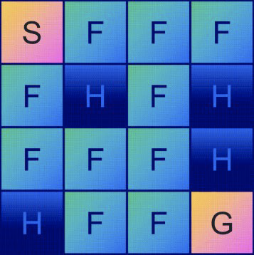
Figure 1. 4x4 Frozen Lake

First, we use the open source to construct the environment as 4*4 frozen lakes. S is the start point, G is the goal, F is the frozen surface, which is safe for the agent to pass, and H means a hole that will prevent the agent from passing. Our method is to use a q-learning algorithm to find an optimal path from start to goal for the agent. The agent has four possible movements: LEFT, DOWN, RIGHT, and UP. The agent must learn to avoid these ice holes to reach the goal in a minimal number of actions. In our environment, there are 16 tiles, from which we can define 16 different states for the agent. In order to know the best action in each state, we can assign a quality value to the action. In this way: 16 states * 4 different actions equal to 64 values. In the Q-learning algorithm, we use a Q-table, in which row contains every state s and the column contains every action a. In the Q-table, each cell list a value Q(s,a), which is the value of action a in a given state. In this way, 1 means the good action, 0 means bad. The agent only gets a reward by 1 if it reaches the goal, then the values in the q-table will be updated based on such an equation:

\( Qn (st, at) = Q(st, at) + α ∙ (ra + γ∙ maQ(st+1, a) − Q(st, at)) \)

Where,

1. The rate \( α \) at which we should modify the initial value of Q(st at) is known as the learning rate. Particularly, the learning rate is a hyperparameter that can be customized and is used to train neural networks. Its value is typically small and positive, falling between 0.0 and 1.0 [7]. The learning rate was not constrained by our research methodology, hence =1. The action will occur too quickly in real life, however, if there are no constraints since the reward value of the subsequent state will quickly outweigh the current value. We do need to strike a balance between imposing restrictions and not doing so.

2. \( γ \) , How much the agent cares about rewards in a reinforcement learning process is determined by the discount factor, which ranges from 0 to 1 [8]. Since there is only one possible reward at the end of the game, we desire a high discount factor in Frozen Lake.

We can solve the maze problem using these two rates. However, the solution might not be the optimal one. The agent will always choose to act to get the highest reward. As a result, the agent will not explore its surroundings, and no q values were added to the q table. In this way, even if the agent can reach the goal, the training process and success rate are not optimal. As a result, we add a new parameter named epsilon to our code to balance the exploration and exploitation tradeoff. Exploration means choosing the actions randomly, and exploitation means acting with the highest value. On one hand, if the agent only focuses on exploration, the training is pointless. On the other hand, if the agent only focuses on exploitation, it can never try new solutions. We want our agent to first explore the environment as much as possible; then, as training goes on, it can focus more on exploitation. Using our new parameter, we defined that when the agent starts acting, it has a probability of \( ε \) to choose action randomly and \( 1−ε \) to choose the action with the highest reward. Through our method, we still have two kinds of decay: the first is linear decay, and the second is exponential decay. The formula we used in our code is shown below:

\( εn = ε ∙ λepisode \)

\( λ = √0.001 \)

\( ε=− λ.episode+εmax \)

\( λ=\frac{1}{total episode} \)

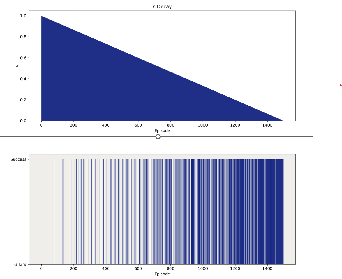
Figure 2. Linear Decay vs Exponential Decay

Figure 2 shows two kinds of decay, we can see clearly that exponential decay occurs more quickly to reach exploration. We will discuss more results afterwards. In our research, we implemented our strategy in a more complicated environment, the 8*8 grid, which means the chance to reach the goal is much smaller than the chance for a 4x4 grid. At the same time, our q-table also expanded to 64x4. Therefore, we plan to use 250,000 episodes to train our agent.

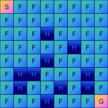
Figure 3. 8x8 Frozen Lake

4.   Results

After training the agent multiple times in two different environments, we got the results as we had first excepted. The cells of the table Q(s,a) represent the total expected reward r of performing that action from the state [9]. From our results table in Figure 4, we can see our strategy works. From the figure, the q-table without the exploration-exploitation tradeoff is very sparse. Both q- tables with linear decay and exponential decay show good exploration of the environment. Therefore, the exploration-exploitation tradeoff is important. It helps the agent understand the environment much better and find multiple optimal solutions.

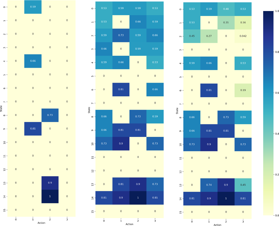
Figure 4. Q-table for No Exploration-Exploitation Tradeoff (Left), Linear Decay (Mid), and Exponential Decay (Right) [4x4 Frozen Lake]

Figure 5 shows the training outcomes for linear decay and exponential decay. Solid blue lines represent success, dashed lines mean failure. We can see that, at first, the agents are more likely to fail. However, as training goes on, the agents start to learn and are more likely to succeed. Also, compared to a linear one, exponential decay is more likely to get successful results. For more complicated mazes showed in figure 6, the exponential decay shows better results. We guess what makes the exponential decay method perform better is that it decays faster in the middle of training. This gives the agent a higher probability of exploitation. In this way, exponential decay will produce better results than linear decay.

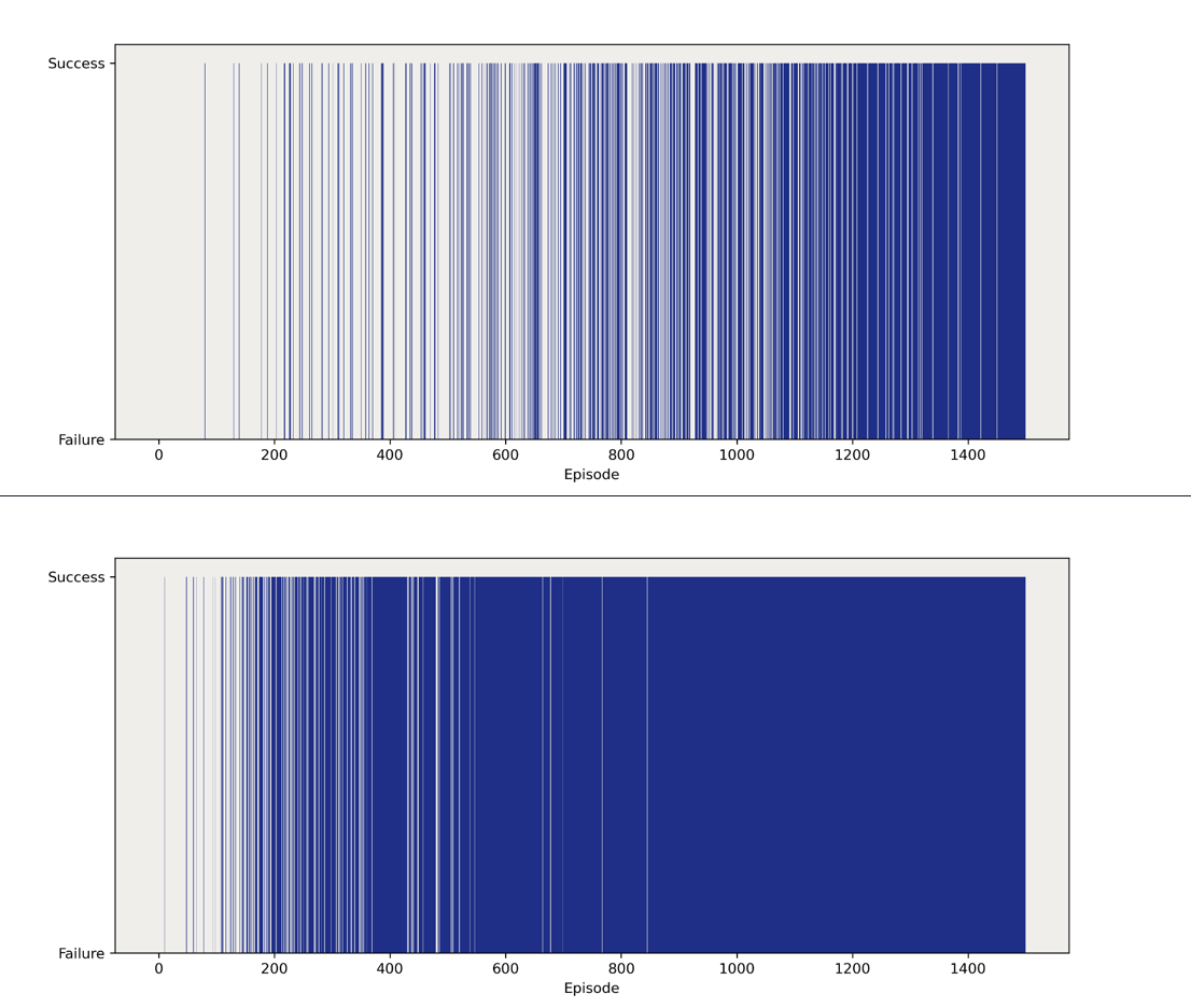
Figure 5. Outcomes for Linear Decay and Exponential Decay (4x4 Frozen Lake)

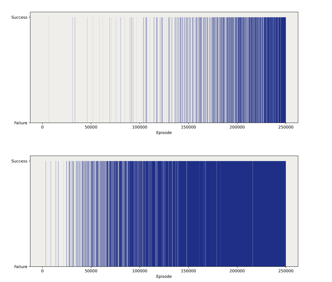
Figure 6. Outcomes for Linear Decay (Up) and Exponential Decay (Below) [8x8 Frozen Lake]

4. Discussion

Through the whole research, our goal is aimed to find a better way to expedite the training speed of the agent in the Q-learning algorithm. We simulated two different environments: one is simple maze, and another is a more complicated one. However, we found the agents were more willing to get a higher reward instead of exploring the environment. To balance the exploration and exploitation tradeoff, we added a new parameter epsilon to our code. Exploitation is defined as a very greedy method in which agents try to get more reward by using the estimated value but not the actual value. So, in this way, agents make the best action decision based on current information [10]. Unlike exploitation, in exploration, agents are more willing to seek for more information to make the best decision based on the whole data. In this way, we defined a new parameter, epsilon, to balance the tradeoff. In our strategy, at first, we set our exploration and exploitation rates to one. When agent starts and learns more and more about the environment, our new parameter epsilon will decrease by some rate, leading to less and less exploration of the environment. In this situation, the agent becomes greedy again for exploiting the environment.

As part of our research, we found that using our new strategy, the training process became more quickly. Also, we found there are two types of decay for epsilon: a linear decay and an exponential decay. As discussed before, this kind of decay is caused by our strategy. The results showed that the exponential decay have more better training process, However, the reason we still did not have enough resources to find out. We assume that the reason why exponential has better training results is because the curve will curve down at the middle of the process, which means the agent will more quickly switch to greedy for higher rewards. The assumption may be proved by the results of later research.

In the future, the author will do more research about why exponential decay will have better results. However, the previous finding is not determined by various complex environment. For my research, the author only simulate two types of maze environment which is not enough to get reliable results. Next step, the author will implement exploitation-exploration tradeoff strategy in more amount of environment and see the different results of epsilon decay. In this way, the author can have more data-based results to show whether the exponential decay will have a better result or not. And using these data, the author can have a better understanding about the efficiency of exploration-exploitation strategy in different circumstances.

5. Conclusion

To wrap up, we can conclude that the exploitation and exploration trade off can speed up the training process. In a more complete maze problem, we found that the exponential decay has better results. The exploitation and exploration method did speed up the learning process by increasing the learning rate and better the decision-making to prevent the agent become too greedy. During our research, we still need to learn more about the difference between linear decay and exponential decay. Our group only used a mathematical method to estimate the reason why exponential has better results. In the future, we will do more research on why exponential decay can have better results and implement more environment to test our method to get a more reliable and data-based results.

References

[1]. Bhatt, S. (2019, April 19). Reinforcement learning 101. Medium. Retrieved August 23, 2022, from https://towardsdatascience.com/reinforcement-learning-101-e24b50e1d292
[2]. Christopher John Cornish Hellaby Watkins. “Learning from Delayed Rewards”. PhD thesis. Cambridge, UK:King’s College, May 1989. Online: http://www.cs.rhul.ac.uk/~chrisw/new_thesis.pdf.
[3]. Epsilon-greedy algorithm in reinforcement learning. (2022, August 23). Retrieved November 15, 2022, from: https://www.geeksforgeeks.org/epsilon-greedy-algorithm-in-reinforcement-learning/
[4]. Solving a maze with Q learning. MitchellSpryn. (n.d.). Retrieved August 23, 2022, from: http://www.mitchellspryn.com/2017/10/28/Solving-A-Maze-With-Q-Learning.html
[5]. Baeldung. (2022, November 11). Epsilon-Greedy Q-Learning. Retrieved November 15, 2022, from: https://www.baeldung.com/cs/epsilon-greedy-q-learning
[6]. Q-learning for beginners. train an AI to solve the frozen lake… | by ... (n.d.). Retrieved November 15, 2022, from: https://towardsdatascience.com/q-learning-for-beginners-2837b777741
[7]. Brownlee, J. (2019, August 06). How to configure the learning rate when training deep learning neural networks. Retrieved November 15, 2022, from: https://machinelearningmastery.com/learning-rate-for-deep-learning-neural-networks/#:~:text=The%20amount%20that%20the%20weights,range%20between%200.0%20and%201.0.
[8]. KarnivaurusKarnivaurus 6, PolBMPolBM 1, Clwainwrightclwainwright 32122 silver badges33 bronze badges, Neil GNeil G 14.1k33 gold badges4343 silver badges8787 bronze badges, Zhenlingcnzhenlingcn 19944 bronze badges, & Shivam KhandelwalShivam Khandelwal 1111 bronze badge. (1963, September 01). Understanding the role of the discount factor in reinforcement learning. Retrieved November 15, 2022, from: https://stats.stackexchange.com/questions/221402/understanding-the-role-of-the-discount-factor-in-reinforcement-learning#:~:text=The%20discount%20factor%20essentially%20determines,that%20produce%20an%20immediate%20reward.
[9]. Arnold, K. (2022, April 11). Q-Table Reinforcement Learning. Retrieved November 15, 2022, from: https://observablehq.com/@kcarnold/q-table-reinforcement-learning
[10]. Exploitation and exploration in machine learning - javatpoint. www.javatpoint.com. (n.d.). Retrieved October 4, 2022, from: https://www.javatpoint.com/exploitation-and-exploration-in-machine-learning
Cite this article
Xu,C. (2023). Maze solving problem using q-learning. Applied and Computational Engineering,6,1491-1497.
Data availability
The datasets used and/or analyzed during the current study will be available from the authors upon reasonable request.
Disclaimer/Publisher's Note
The statements, opinions and data contained in all publications are solely those of the individual author(s) and contributor(s) and not of EWA Publishing and/or the editor(s). EWA Publishing and/or the editor(s) disclaim responsibility for any injury to people or property resulting from any ideas, methods, instructions or products referred to in the content.
About volume
Volume title: Proceedings of the 3rd International Conference on Signal Processing and Machine Learning
© 2024 by the author(s). Licensee EWA Publishing, Oxford, UK. This article is an open access article distributed under the terms and
conditions of the Creative Commons Attribution (CC BY) license. Authors who
publish this series agree to the following terms:
1. Authors retain copyright and grant the series right of first publication with the work simultaneously licensed under a Creative Commons
Attribution License that allows others to share the work with an acknowledgment of the work's authorship and initial publication in this
series.
2. Authors are able to enter into separate, additional contractual arrangements for the non-exclusive distribution of the series's published
version of the work (e.g., post it to an institutional repository or publish it in a book), with an acknowledgment of its initial
publication in this series.
3. Authors are permitted and encouraged to post their work online (e.g., in institutional repositories or on their website) prior to and
during the submission process, as it can lead to productive exchanges, as well as earlier and greater citation of published work (See
Open access policy for details).