Improved Time-aware Debiasing Models for Recommender Systems

Sitan Wang¹⁺, Xinyi Wu²⁺, Lintong Zhao³⁺, Yuru Xue^4+*, Ruihan Xia⁵⁺, Zhuofan Sun⁶⁺

¹Cranbrook Schools, Bloomfield Hills, USA, swang25@cranbrook.edu 

²International School of Information Science & Engineering, Dalian University of Technology, Dalian, China, woo.xinyi.woo@gmail.com

³Dalton Academy, The Affiliated High School of Peking University, Bejing, China, lintong_zhao@163.com

⁴College of Engineering and Computer Science, The University of Sydney, Sydney, Australia, aaxue36120@gmail.com

⁵College of Letter and Science, University of California, Berkeley, Berkeley,USA, ruihan.xia@berkeley.edu

⁶Bejing-Dublin International College, University College Dublin, Dublin, Ireland, zhuofan.sun@ucdconnect.ie

+These authors contributed equally. The order determined by free-rolling dice.

*Corresponding author email: aaxue36120@gmail.com

Abstract—Recommender systems are affected by user selection bias during user interactions. Previously, Huang, Jin et al. proposed the TMF-DANCER model to deal with the fact that selection bias is dynamic, and the popularity of an item and user preferences may change drastically over time. However, the previous time-aware methods did not consider the continuity of time, and performing collaborative filtering with matrix factorization may not be able to capture the complex structure of user interaction data. Our methods enhance the effectiveness of time-aware debiasing by utilizing the time-varying sequential method to alleviate the discontinuity of time-based on the frequency-based method, Replacing the matrix factorization with neural collaborative filtering (NCF). We used movie lens 100k as the data for training. The experimental results indicate that methods incorporating the time-varying sequential method and NCF have better performance in rating prediction than debiasing methods without.

Keywords—Selection bias, Dynamic user preferences, Time-varying sequential method, Time-aware Neural Collaborative Filtering

1. Introduction

User behavior data is observational rather than experimental. This brings a very large number of biases, typically: selection bias, exposure bias, position bias, conformity bias, and popularity bias, etc. If the data is fitted blindly without considering the inherent biases, it will lead to many serious problems, such as inconsistency between offline evaluation and online metrics, damaging users' satisfaction and trust in the recommended service, etc. But there are some advances in research that address different biases now.

One paper in the area of proving bias changes over time is 'It Is Different When Items Are Older: Debiasing Recommendations When Selection Bias and User Preferences Are Dynamic'. This paper demonstrates that in the real world, time-aware methods can predict selection bias better than static methods [1]. However, it does not consider biases that depend on the previous bias. In other words, biases should depend on each other.

In addition, the paper uses Matrix Factorization (MF) for collaborative filtering. Compared to traditional machine learning techniques, especially MF, deep learning models can dig out more hidden patterns in data. Neural Collaborative Filtering (NCF) uses neural network layers to replace the simple inner product of user and item vectors. Moreover, MF applies to NCF models, or NCF is a generalized matrix factorization model.

In 2017, a group of scholars published a paper on neural collaborative filtering. By analyzing two real-world datasets, they demonstrated that their proposed NCF framework is significantly more efficient than the current state-of-the-art methods under evaluation through HR@10, and NDCG@10. In addition, researchers have found that neural networks with deeper layers perform better at recommending products [2].

Based on the above, ignoring time continuity might affect the functionality of time-aware debiasing models. Moreover, MF appears to be primitive compared to state-of-the-art models. Thus, using a method to mitigate the discontinuity of frequency-based methods on time, and substituting the MF with NCF in the time-aware situation, is a reasonable improvement to the debiasing method proposed by Huang, Jin, et al.

According to the current problems, this work has made the following significant contributions:

(1) We proposed a time-varying sequential method to cope with the discontinuity of time in current time-aware debiasing methods. Moreover, we used neural collaborative filtering as a substitute for matrix factorization in time-aware situations.

(2) We find that deep learning method in recommender systems such as NCF show better performance than matrix decomposition MF. (RQ1)

(3) Experimental results suggest that the time-varying sequential method will improve the accuracy of the propensity prediction. (RQ2)

(4) When embedding size alters from 3 to 6, MF-based and NCF-based time-varying methods perform relatively better with an embedding size of 4. (RQ3)

(5) We performed sensitivity analysis on alpha and beta for the time-varying sequential method and; the learning rate of optimizer for the NCF-based method. (RQ4)

2. Introduces Bias and Existing Studies

This chapter will mainly explain all the different biases the recommender system needs to cope with. We also add in the current research progress in each field to demonstrate how far the research has progressed.

2.1 Selection Bias

Selection bias mainly comes from explicit feedback from users, such as ratings of items. Since users tend to rate items they are interested in, and rarely rate items they are seldom uninterested in, resulting in the problem of Missing Not at Random (MNAR), the observed ratings are not all ratings. A representative sample of, resulting in selection bias.

This paper proposes using an Inverse Propensity Score (IPS) to deal with selection bias. The propensity score can be considered the probability that each piece of data is observed. In this paper, the recommendation problem is viewed from the perspective of causal inference, arguing that exposing a user to a particular product in a recommendation system is similar to imposing a specific treatment on a patient in medicine. Both tasks have in common that only a few patients (users) are known to respond to a few treatment modalities (items), while the outcome of most patient-treatment (user-item) pairs is not observed [3].

2.2 Exposure Bias

Exposure bias mainly comes from implicit feedback from users, such as clicks. Users can only see a part of the items the system exposes and make clicks and other reactions. However, interactions that are not included in the data do not necessarily mean that the user does not like it. It is also possible that the user does not know the item.

Although the observed click behavior in a recommender system can reflect user preferences to some extent, missing click data does not necessarily mean negative feedback from users, and it is also possible that users do not see these items at all (Positive-unlabeled problem), which poses difficulties in predicting user preferences from implicit feedback. To cope with the above problems and to solve the MNAR problem of recommender systems, this paper first assumes that items must be exposed to the user and relevant for a click to occur. Second, an ideal loss function is defined to achieve the recommendation task by maximizing relevance.

Based on the propensity score approach, an unbiased estimator of the ideal loss function is proposed in this paper. In this paper, it is theoretically demonstrated that when the propensity score is too small (e.g., some items are too underexposed), the unbiased estimator generates a large variance, so we propose to improve the unbiased estimator by trimming the propensity score to prevent it from being too small. Experiments on semi-synthetic and real datasets demonstrate that the proposed method outperforms the models involved in the comparison, especially in improving the recommendations for items that rarely appear in the training set (items with low exposure) [4].

2.3 Position Bias

Position bias refers to the tendency of users to interact (click, buy, etc.) with items at the top of the recommended list, even though these items may be irrelevant or not the most preferred. This results in interacting items that may not be highly relevant.

Unlike web search, where users usually click on the top pages, in Feeds Recommendation, users are more likely to keep scrolling down to see more items, as in shopping sites where they keep scrolling down to browse items. Since the display information of items affects users' judgment, the ranking method based on the observed implicit feedback data is biased. In addition to location bias, this paper proposes that context bias (Context bias) is more significant than location bias when users browse deeper, arguing that the probability of users interacting with items at this time is influenced by the contextual environment in which the items are displayed. The click rate is higher when the target item is surrounded by items that are not very similar.

To remove location and context bias, i.e., Context-aware position bias, this paper proposes an unbiased ranking learning framework, assuming that the probability of a user clicking on an item is influenced by three factors, namely, Examination, Relevance, and Comparison. The propensity score considering the combination of these three bias factors is first defined. Then the propensity score is estimated using a regression-based expectation maximization algorithm, and the propensity score is evaluated directly and indirectly by balancing inspection and ranking metrics. The advantage of introducing contextual biases on top of positional biases is experimentally demonstrated on a real e-commerce dataset [5].

2.4 Unfairness Bias

Unfairness bias is when the system mistreats some individuals or groups in favor of other users. For example, in some job recommendation systems, women may be less likely to be recommended for advertisements such as higher salaries or career guidance services than men, creating gender inequity.

First, as shown in Figure 1, a deep neural network is pre-trained on a large amount of implicit feedback data involving non-sensitive items to solve the acute data sparsity problem (e.g., users usually have only one or two professions or positions). Then, the bias of the user vectors learned in the previous step is reduced using a method commonly used in previous work to remove the bias of word vectors. They were finally fine-tuning (Fine-tuning) of the neural network using sensitive data and adding a fairness penalty term to the objective function to achieve sensitive item recommendations.

This paper uses two kinds of bias correction: the bias brought by non-sensitive items to the input vector and the bias brought by sensitive items to the prediction output. Experiments on a dataset containing both sensitive and non-sensitive information demonstrate that bias interventions are essential for fairness recommendation [6].

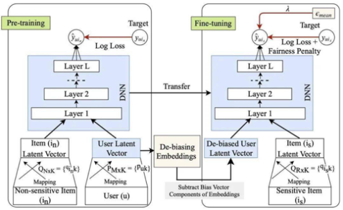
Figure 1: Neural Fair Collaborative Filtering Framework (NFCF) (Islam, Rashidul & et al, 2021) [6]

3. Formulate Debias Problem

Our paper will mainly focus on debiasing the selection bias. Below are some existing methods to deal with the problem.

3.1 IPS Estimator

Schnabel et al. proposed the use of an Inverse Propensity Score (IPS) to deal with selection bias [7]. A toy example is adapted from Steck (2010) to illustrate how selection bias can ruin conventional evaluation when used with a set of held-out ratings [8]. With \( u∈\lbrace 1,…,U\rbrace \) denote the users; with \( i∈\lbrace 1,…,I\rbrace \) denote the movies. The matrix of true ratings is denoted by \( Y∈{ℛ^{U×I}} \) . The propensity score can be considered the probability that each piece of data will be observed. This paper looks at the recommendation problem from the perspective of causal inference, arguing that exposing a user to a product in a recommendation system is like imposing a certain treatment on a patient in medicine. What both tasks have in common is that only a small number of patients (users) are known to respond to a small number of treatment modalities (items), while the outcome of most patient-treatment (user-item) pairs is not observed. The article specifies the ideal evaluation method, i.e., the standard evaluation indicators when all user-item pairs are observable.

\( R(\hat{Y})=\frac{1}{U\cdot I}\sum _{u=1}^{U}\sum _{i=1}^{I}{δ_{u,i}} (Y,\hat{Y}) (1) \)

Second, it is proposed to construct an unbiased estimator of the ideal rubric, IPS Estimator, using inverse propensity scores to weigh the observed data.

\( {\hat{R}_{IPS}}(\hat{Y}|P)=\frac{1}{U\cdot I}\sum _{(u,i): {O_{u,i}}=1}\frac{{δ_{u,i}}(Y,\hat{Y})}{{P_{u,i}}} (2) \)

In addition, the paper introduces two methods for predicting propensity scores (plain Bayesian, logistic regression) and proposes a matrix decomposition model based on propensity scores (MF-IPS) for recommendation tasks. Experiments on semi-synthetic and real datasets, respectively, demonstrate that IPS estimator is an unbiased estimator of the ideal rubric and that the MF-IPS model outperforms traditional matrix decomposition algorithms for the purpose of removing selection bias.

3.2 DR Estimator

Both types of methods form the previous method for dealing with selection bias - data padding and propensity scores - have certain limitations: data padding-based methods can lead to bias because they cannot accurately predict the data; propensity score-based methods suffer from large variance because propensity scores are difficult to be accurately estimated.

In order to remove these two limitations, this paper proposes a doubly robust way of constructing an unbiased estimator (DR Estimator) using a combination of the above two methods, achieving the aim that the DR estimator is unbiased as long as one of the two methods is accurate. Given the inferred error of data filling and the learned propensity score, the objective function based on the DR estimator is defined as:

\( {ε_{DR}}={ε_{DR}}(\hat{R, }{R^{o}})=\frac{1}{|D|}\sum _{u,i ∈D}({\hat{e}_{u,i}}+\frac{{o_{u,i}}{δ_{u,i}}}{{\hat{p}_{u,i}}}) (3) \)

When using DR estimator for recommendation learning, there is a need to avoid inferential errors introduced by the data-population model from impairing the training of the recommendation model. In this paper, a generalization bound is designed to analyze this problem and observe how the errors affect the accuracy of the prediction model using DR estimator. To achieve effect guarantees, an additional joint learning approach is proposed based on the DR estimator, where the parameters of the padding model are learned while minimizing training losses to improve the prediction accuracy of the model. Experiments on four real datasets validate the effectiveness of this robust dual estimator and joint learning approach.

3.3 Deblasing Recommendations in the Dynamic Scenar (Dancer)

Existing methods of eliminating selection bias (hotness bias) treat the bias as static. However, both item hotness and user preferences change over time. This is the reason Huang et al. proposed DANCER which is a time-varying IPS. DANCER is defined as:

\( {ℒ_{DANCER}}=\frac{1}{|U|·|ℐ|·|T|}\sum _{u,i,t:{o_{u,i,t=1}}}\frac{L({ŷ_{u,i,t}},{y_{u,i,t)}}}{{P_{u,i,t}}}(4) \)

This paper proposes an improved method based on IPS to consider the dynamic changes in item hotness and user preferences, and it is the first attempt in this direction. However, this paper is only an attempt at collaborative filtering. Dynamic deviations, being time-dependent, should be most associated with sequential recommendations.

4. Propensity Estimation Methods

\( {p_{u,i,t}}=P({O_{u,i,t}}=1 | X, {X^{ℎid}}, Y)(5) \)

With the different methods to predict \( \hat{Y} \) , the estimated user’s rating, it is also important to have a good method to estimate the propensity. To estimate propensity is to estimate the probability \( {p_{u,i,t}} \) with which rating of user \( u  \) , item \( i  \) and time \( t  \) , in a time-varying case, will be observed. The equation for propensity will be dependent on some observed feature \( X  \) , unobserved feature \( {X^{ℎid}} \) , and the ratings \( Y  \) [3].

\( {p_{u,i,t}}=P({O_{u,i,t}}=1 | X, {X^{ℎid}}, Y)（6） \)

The following provides several different ways to estimate this propensity in both static and time-varying scenarios.

4.1 Propensity Estimation without the time effect

The propensity estimated without the time effect can be used in IPS and DR Via Naïve Bayes. The first method assumes that propensity’s dependency on \( X, {X^{ℎid}} \) is negligible, so the propensity equation can be reduced to

\( {p_{u,i = }}P({O_{u,i}}=1 | Y)(7) \)

We also can neglect the variable \( t  \) as this is in a static case. We can treat \( {Y_{u,i}} \) as observed, since we only need the propensities for observed entries to compute IPS and DR [3]. This is the Naive Bayes propensity estimator:

\( P(O=1 | Y=r)=\frac{P(Y=r | O=1) P(O=1)}{P(Y=r)}(8) \)

All the subscripts are dropped, but \( u,i  \) are all carried over every \( Y  \) and \( O  \) in the equation. \( Y=r  \) represents there is a rating for the given Y. \( P(Y=r | O=1) \) and \( P(O=1) \) can be easily obtained by counting from a given MNAR data. \( P(Y=r) \) , however, would require a small sample of MCAR data.

Via Logic Regression. The second approach is based on logic regression which doesn’t require a sample of MCAR data. It aims to find a parameter \( φ  \) such that \( O  \) will be independent of \( {X^{ℎid}} \) and \( Y  \) , so equation to calculate propensity can be simplified to \( {p_{u,i}}=P({O_{u,i}}=1 | X, φ) \) [3]. If we have this \( φ=(w,β,γ) \) , then we can calculate the propensity:

\( {p_{u,i}}=σ({w^{T}}{X_{u,i}}+{β_{i}}+{γ_{u}})(9) \)

\( { X_{u,i}} \) is a vector containing all user-item pairs. \( {β_{i}} \) and \( {γ_{u}} \) are offsets for item and user respectively, and \( σ  \) is representing the sigmoid function to cast the data onto 0-1 scale.

The propensity estimated using these two methods can be used for IPS and DR as both of the methods don’t include time variable in the calculation. In the next section, we will explain some propensity estimation methods that take time into account.

4.2 Propensity Estimation with the Time Effect

Huang et al. proposed eight different methods to estimate propensity in a time-varying scenario [1]. They use \( σ  \) to denotate the sigmoid function. All bolded letters are trained embedding vectors of user, item or time based on the subscript.

(1) Constant: This method assumes that there is no bias and is purely the fraction of all ratings. The propensity will be the same for each user \( u  \) , item \( i  \) , and time \( t  \) :

\( {p̂_{u,i,t}}=\frac{\sum _{u \prime ∈U}\sum _{t \prime ∈E}{o_{u \prime ,i,t \prime }}}{|U|·|ℐ|·|T|} (10) \)

Static Item Popularity (Pop): This method assumes that there is no bias over users and time periods as this method has a propensity for every given item. The propensity calculated will be a fraction of an item \( i  \) ’s all rating. The propensity will be the same for each user \( u  \) and time \( t  \) for an item \( i  \) :

\( {p̂_{u,i,t}}=\frac{\sum _{u \prime ∈U}\sum _{t \prime ∈E}{o_{u \prime ,i,t \prime }}}{|U|·|T|}(11) \)

(2) Time-aware Item Popularity (T-Pop): This method is defined as the fraction of all ratings that have been given to item \( i  \) on time \( t  \) . The propensity will be the same for every user for an item \( i  \) on time \( t  \) :

\( {p̂_{u,i,t}}=\frac{\sum _{u \prime ∈U}{o_{u \prime ,i,t}}}{|U|}(12) \)

(3) Static Matrix Factorization (MF): This method is purely a standard matrix factorization model that assumes selection bias is static:

\( {p̂_{u,i,t}}=σ(p_{u}^{T}{q_{i}})(13) \)

(4) Time-aware Matrix Factorization (TMF): This method is an improvement from the plain MF as it can capture the drift as an item gets older by adding a constant bias \( {b_{t}} \) :

\( {p̂_{u,i,t}}=σ(p_{u}^{T}{q_{i}}+{b_{t}})(14) \)

(5) Time-aware Tensor Factorization (TTF): TTF is another variant of MF as it uses element-wise multiplication to mimic the effect of time on an item:

\( {p̂_{u,i,t}}=σ(p_{u}^{T}{(q_{i}}×{a_{t}}))(15) \)

(6) TTF++: TTF++ is a modification of TTF as it changes multiplication to summation instead:

\( {p̂_{u,i,t}}=σ(p_{u}^{T}{(q_{i}}+{a_{t}}))(16) \)

(7) Time-aware Matrix & Tensor Factorization (TMTF): Finally, they proposed TMTF which combines TMF and TTF++ together:

\( {p̂_{u,i,t}}=σ(p_{u}^{T}{(q_{i}}+{a_{t}})+{b_{t}})(17) \)

Our methods will mainly be improving these time-varying propensity estimation methods they propose as ours will better mimic the real-life scenario and have a higher accuracy.

5. Time-Dependent Methods

The eight methods proposed by Huang et al. can be divided into two sections according to the method they are based on: observation matrix and matrix factorization. Accordingly, we proposed two ideas which will improve their methods, and they are time-varying sequential method and time-aware neural collaborative filtering. We unfortunately can’t improve Pop anymore since it’s static for every item, and if we add the time variable into Pop, it will become the same with T-Pop. Below, we will describe how we can improve their methods in detail.

5.1 Time-varying Sequential Method (TS)

Constant and T-Pop are the two that use observation matrix. The problem with these two methods is that the time periods are independent from each other. The propensity calculated using either of the methods is only based on the current time period. However, this isn’t the case in real-life example: people’s interests from yesterday can affect what people favor today which means each time period should be dependent on the previous ones. From this theory, we devise an equation to mimic the behavior:

\( {p_{u,i,t}}=β{p_{u,i,t−1}}+α{(p_{u,i,t}}−{p_{u,i,t−1}})(18) \)

The calculation for propensity won’t change, but we gave weight to the previous time period, so the previous propensity will affect the current propensity. \( β  \) and \( α  \) are two hyper-parameters that together control how much we should trust the propensity: if \( β  \) is larger, it means we trust the previous propensity more, else otherwise.

5.2 Time-varying Neural Collabrative filtering (NCF)

Time-varying Neural Collaborative Filtering (TNCF) that we proposed, builds on the framework of NCF that is demonstrated in the figure below:

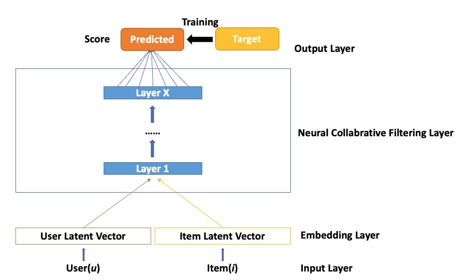
Figure 2: Neural Collaborative Filtering Framework

It is constructed with the input layer, embedding layer, NCF layer, and output layer. In this work, there are two feature vectors in the input layer that describe user u and item i, only user and item identities are used as input features, then transforming them to a binarized sparse vector. The embedding layer lies above the input layer, it's a fully connected layer that translates sparse vectors into a dense representation. The obtained user (item) embedding can be identified as the latent factor, and they are then passed into a multi-layer neural architecture, namely, the NCF layer. NCF layers can be customized to discover certain latent structures of interaction between a user and an item. The final output layer is the predicted score, and training is conducted by minimizing the loss between predicted score and its target value. Thus, the formulated NCF predictive model can be described as:

\( {\hat{y}_{ui}}=f(u,i|Θ）(19) \)

Where \( Θ  \) represents the parameters. Function f here refers to the NCF layer, where Multi-Layer Perceptron (MLP) can be placed. NCF uses two paths to model users and items, and then concatenate the two. But simple concatenation does not take into account the interaction between users and items. To solve this problem, a hidden layer is added to learn the interaction between user and item, not just the element-wise product that Generalized Matrix Factorization (GMF) takes.

MLP layers can freely choose activation functions, such as sigmoid, hyperbolic tangents (tanh), and Rectifiers (ReLU). However, according to “Neural collaborative filtering”[2], ReLU tends to perform the best among those three above. ReLU is more biologically plausible and has been shown to not lead to oversaturation; in addition, it supports sparse activations, which are well suited for sparse data so that the model does not overfit. One thing to note is that their study also proves the necessity of pretraining the performance of the models.

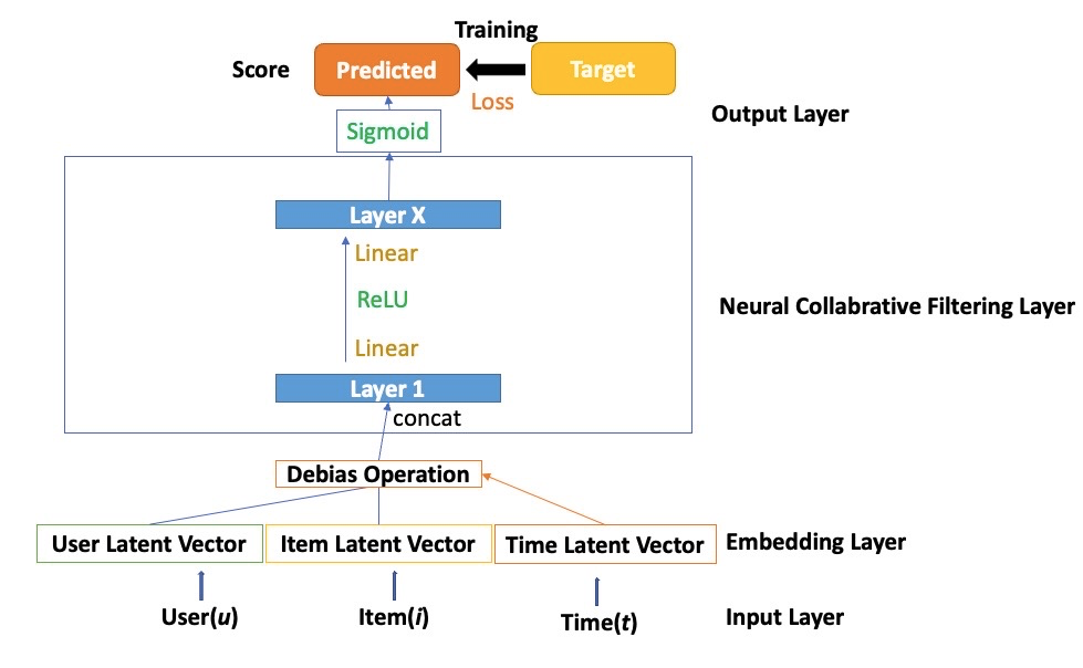
Figure 3: Time-aware Neural Collaborative Filtering Framework

Procedures of TNCF differ from the NCF framework by debiasing user, item embedding(s). It can also be interpreted as debiasing the embedding layer with interaction information obtained in the time index. There can be multiple time-aware debiasing approaches as mentioned in chapter 4, specifically TMF, TTF, TTF++, TMTF, which is later transformed into TNCF, TTNCF, TTNCF++, and TNTCF correspondingly.

6. Experiments

6.1 RQ1: Is the NCF Time-Varying Method More Effective than the MF Time-Varying Method?

To answer RQ1: Is the NCF Time-Varying method more effective than the MF Time-Varying method? we evaluate how adapting matrix factorization methods into neural collaborative filtering affects the prediction of propensity.

6.1.1 Experiment Setup for RQ1

Based on users u, items i, and item-ages t, the predicted probability is compared to observed propensity in dataset. Our comparison is based on 5 pairs of methods. Five MF based methods have been introduced in previous chapters. Below are five neural collaborative filtering methods:

(1) Neural Collaborative Filtering (NCF)

(2) Time-aware Matrix Factorization (TNCF)

(3) Time-aware Tensor Neural Collaborative Filtering (TTNCF)

(4) TTNCF++

(5) Time-aware Matrix & Tensor Factorization (TNTCF)

The main calculation for the propensity will be the same, however our NCF models are going through the different layers of the neural network which digs out more hidden patterns.

We propose to apply Mean Squared Error (MSE) to measure the loss and Area Under a Receiver Operating Characteristic (AUC) to measure the performance of score classifiers. We use Normalized Discounted Cumulative Gain (NDCG@5) to evaluate the quality of recommendation.

MSE: \( {δ_{u, i, t}}(P, \hat{P}) = {({P_{u,i,t }}− {\hat{P}_{u,i,t}})^{2}}(20)  \)

The area under a receiver operating characteristic (ROC) curve, abbreviated as AUC, is a single scalar value that measures the overall performance of a binary classifier [9]. Its value ranges from 0.5 to 1.0. The minimum value represents the performance of a random classifier, and the maximum value represents a perfect classifier.

NDCG@5: NDCG is calculated as:

\( nDC{G_{p}}=\frac{DC{G_{p}}}{IDC{G_{p}}}(21) \)

CG stands for the cumulative gain which sums the gains, the relevance score for each item recommended, of the first p items recommended. To take the ordering into account, discounted cumulative gain (DCG) calculates by the sum of the first p gains with a denominator, \( {log_{2}}{(i+1)} \) , giving more weightage to items recommended at the top. But DCG is still incomplete since the number of recommendations served may vary for every user. Consequently, normalized nDCG, adds a normalization denominator to DCG. The denominator is the ideal DCG score when recommending the most relevant items first. It is computed by:

\( IDC{G_{p}}=\sum _{i=1}^{|REL|}\frac{{2^{re{l_{i}}}}−1}{{log_{2}}{(i+1)}}(22) \)

REL represents the list of relevant documents (ordered by their relevance) in the corpus up to position p.

The same criteria are applied to later discussion in RQ 2, 3, and 4. The results illustrated in tables below are averages of 5 experiments. To control the variable, the performance in RQ1 is based on 4 time periods which are averagely distributed among the span of time.

6.1.2 Results for RQ1

RQ 1: Performance in propensity prediction of MF and NCF with 4 time periods.

Table 1: Comparison between MF methods and NCF methods.

The results for the first research question are in Table 1. For both the use of matrix factorization method and neural collaborative filtering, time-aware methods TMF, TTF, TTF++, TMTF, TNCF, TTNCF, TTNCF++, TNTCF demonstrate lower MSE and higher AUC than base models of MF and NCF respectively. Comparing MF and NCF, each adaptation of NCF performs better than their counterpart in MF. This is probably because multi-layer structure can better capture non-linearity in user-item-time interaction in recommender system. Under the NCF category, TNCF outperforms all other methods.

Therefore, we conclude that NCF Time-Varying methods are more effective than the MF Time-Varying method in predicting propensity in real-world data. The result strongly demonstrates that applying neural network in propensity estimation, at least in the case of recommendation system, can significantly improve efficiency and accuracy.

6.2 RQ2: Does the Time-varying Sequential Method Help with Smoothing?

To answer RQ2: Does the time-varying sequential method help with smoothing? we evaluate whether the time-varying sequential method actually improve the accuracy of the propensity prediction.

6.2.1 Experiment Setup for RQ2

We will use the same measurements as RQ1, MSE, AUC, NDCG@5, to evaluate how close our estimated propensity to the real propensity for the data set. We apply the time-varying sequential method to Constant and T-Pop. Here is the definition for the two:

(1) Time-varying Sequential Constant (TSC): This method is the fraction of all ratings from user \( u  \) , item \( i  \) in time \( t  \) . For time 0, the propensity will be unchanged, but for any other time, the final propensity will need to balance with the propensity from the previous time according to the time-varying sequential method.

(2) Time-varying Sequential Item Popularity (TS-Pop): The second method is the fraction of all ratings from user \( u  \) in item \( i  \) and time \( t  \) . For every item \( i  \) , excluding every propensity in time 0, the current propensity will be updated based on the weights on previous propensity and the current propensity calculated from original T-Pop method.

All the results are based on the mean of 5 same runs.

6.2.2 Results for RQ2

Table 2 displays the performance of Constant, TSC, T-Pop and TS-Pop. We can easily see that our proposed methods, TSC and TS-Pop, have a lower MSE, higher AUC and NDCG@5, which means that our methods perform better. In addition, since the TS method is only adding a linear time to the algorithm, the overall time will not change drastically.

Finally, we can answer RQ2 in affirmative: our newly proposed TS method truly performs better than the time-varying methods around the same time.

Table 2: Comparison between time-varying methods and time-varying sequential methods.

6.3 RQ3: How does Embedding Size Influence MF and NCF Time-varying Methods?

To answer RQ3: How does embedding size influence MF and NCF time-varying methods? we fix other parameters unchanged, only change the embedding size, and conduct experiments.

6.3.1 Experimental Setup for RQ3

The variation interval of the embedding size we choose is from 3 to 6. In order to analyze the effect of embedding size, we conducted multiple experiments on the MF-based time-varying methods and the NCF-based time-varying methods respectively, and recorded the corresponding Mean Squared Error (MSE) and Area Under Curve (AUC). For the objectivity and generality of the results, we used the mean of the results of 5 runs for the AUC and MSE of the results under each embedding size.

6.3.2 Results for RQ3

Figure 2 shows the performance of MF (baseline) and 4 time-varying methods based on MF under different embedding sizes. We see that all methods have the highest AUC with an embedding size of 4, except TMF, which has the highest AUC with an embedding size of 3. In addition, when the embedding size is 4, the MSE of the other four methods except TMF also reaches the minimum. Although the AUC and MSE of TMF are not optimal when the embedding size is 4, the best AUC and MSE are obtained when the embedding size is 3 and the embedding size is 5 respectively. Therefore, considering both AUC and MSE, when the embedding size is 4, the performance of TMF beats embeddings of other sizes. Moreover, compared with other methods, TTF++ and TMTF are more sensitive to changes in the size of the embedding.

Figure 3 shows the performance of NCF (baseline) and 4 time-varying methods based on NCF under different embedding sizes. We observe that as the embedding size changes from 3 to 6, the AUC of NCF, TTNCF++ and TNTCF show a gradual upward trend, while the AUC of TNCF and TTNCF tend to remain unchanged after reaching the maximum when the embedding size is 4. In addition, except for NCF and TNTCF, the MSE of all other methods achieves the minimum value when the embedding size is 4. Considering both the AUC and MSE, we believe that the NCF-based time-varying methods perform relatively better when the embedding is 4. Lastly, NCF-based time-varying methods are relatively sensitive to changes in the embedding size.

Finally, we can answer RQ3 in the affirmative: as the embedding size changes from 3 to 6, MF-based and NCF-based time-varying methods perform relatively better with an embedding size of 4.

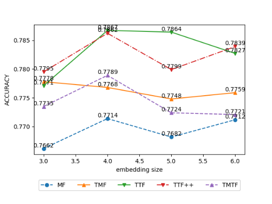
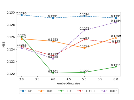
Figure 4: The effect of different embedding sizes on MF time-varying Accuracy (left) and MSE (right).

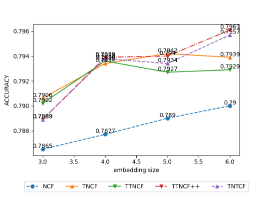
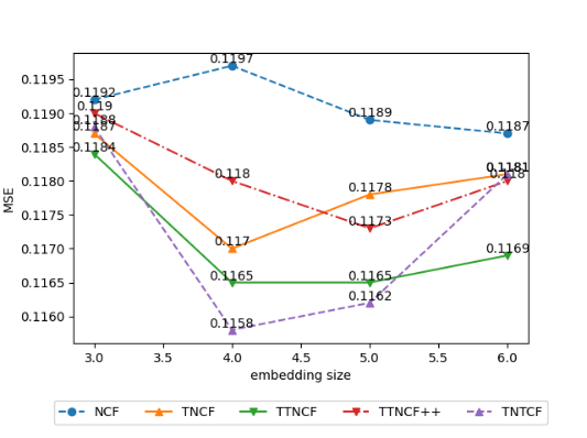
Figure 5: The effect of different embedding sizes on NCF time-varying Accuracy (left) and MSE (right).

6.4 RQ4: Sensitivity Analysis:(1) How does the Time-period Division Method Affect the Results？(2)How does \( α  \) and \( β  \) effect the experiment? (3) How does the learning rate of optimizer affect NCF-based time-varying methods?

To answer RQ4 (1): How does the time-period division method affect the results? we propose a new time-period division method and compare the results of our improved methods under the two different time-period division methods.

Table 3: Performance comparison of different methods in different time-period division methods. ↑/↓indicates whether larger or smaller values are better.

To answer RQ4 (2): How does alpha and beta affect the experiment?, we change alpha and beta several times to find the best result.

To answer RQ4 (3): How does the learning rate of optimizer affect NCF-based time-varying methods?, we fix other parameters unchanged, only change the learning rate of optimizer, and conduct experiments.

6.4.1 Experimental Setup for RQ4

(1) Our new proposed time-period division method divides the time periods into six segments, unlike the previous equal division into four segments: the six-time intervals in our new method are unequally spaced and increase by one in sequence. We conduct experiments where only the time-period division method is different and other parameters are fixed. We run each method five times and record its AUC, MSE and NDCG@5, and take the mean of the five runs as the final result.

(2) We run TS and TS-Pop 5 times each with the same hyper-parameter alpha and beta and take the mean of its AUC, MSE and NDCG@5.

(3) To investigate the effect of different learning rates on the performance of NCF-based methods, we take a set of learning rate (LR) values for multiple experiments. The learning rates we use are from the set LR = {0.001, 0,002, 0,005, 0,006, 0,007, 0.008, 0.009, 0.01, 0,02, 0,05}.

6.4.2 Results for RQ4

The main results of our comparison of different methods using different time-period division methods are displayed in Table 3. Based on the displayed results we can make 4 observations:(1) For NCF-based methods, all the other 4 methods except TNCF have better MSE results when using the 4 time-period division method. (2) For NCF-based methods, NCF, TNCF and TNTCF have better AUC results when using the 4 time-period division method, while TTNCF and TTNCF++ have better AUC results when using the 6 time-period division method. (3) For NCF-based methods, NCF and TNTCF have better NDCG@5 when using the 6 time-period division method. (4) In general, for NCF-based methods, the performance changes are relatively small, so we believe that NCF-based methods have strong robustness to different time-period division methods.

Table 4 displays the results of TS and TS-Pop on the different hyper-parameters. By the table, we can clearly tell that when alpha is 0.8 and beta is 0.2, the result for TSC is the best. In the other hand, when alpha is 0.2 and beta is 0.8, TS-Pop performs the best. Alpha and beta are related how much we want to trust the propensity from the previous time period, and from our result we can deduce that TS will better be approximated with the current propensity, and TS-Pop will better be approximated by relying on the previous propensity.

Figure 4 and Figure 5 show the effect of different learning rates of optimizer on the performance of NCF-based methods. We observe that the NCF-based time-varying methods are relatively robust in the range of learning rates of 0.005 to 0.01. All the five methods have high AUC and low MSE in the above learning rate range. However, when the learning rate is lower than 0.005 or larger than 0.01, the performance of the four NCF-based time-varying methods starts to become unstable. We also note that the NCF (baseline) performs well at smaller learning rates, i.e., the NCF is robust over a range of learning rates from 0.001 to 0.01.

Finally, we can answer RQ4 in the affirmative: (1) All our proposed methods are relatively robust to different time-period division methods. (2) Different alpha and beta suits TS and TS-Pop for them to perform the best results. (3) For NCF-based methods, the baseline (NCF) has better performance and robustness when the learning rate is in the range of 0.001-0.01 and the four NCF-based time-varying methods have better performance and robustness when the learning rate is in the range of 0.005-0.01.

Table 4: Performance comparison of different methods with different hyper-parameters ↑/↓indicates whether larger or smaller values are better.

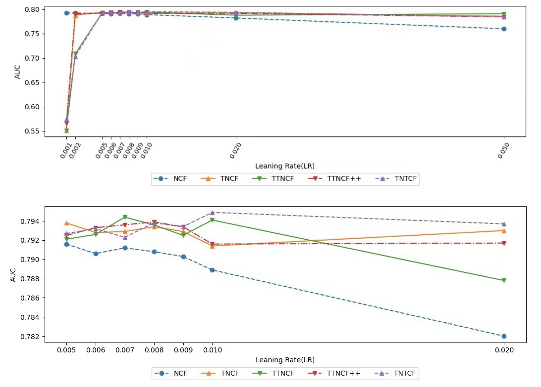
Figure 6: The effect of different learning rates on the AUC of NCF-based methods.

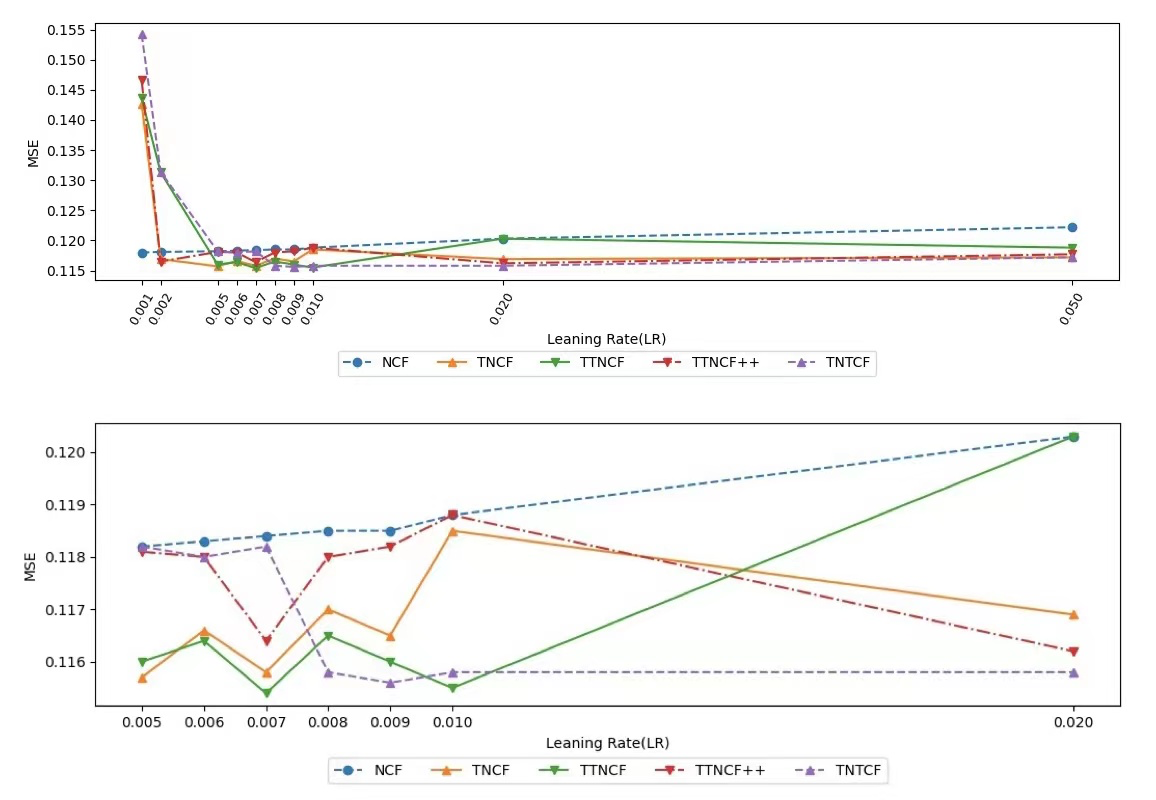
Figure 7: The effect of different learning rates on the MSE of NCF-based methods.

7. Conclusions

The problem that recommender systems are affected by user and item’s dynamic biases during interactions, are previously debiased with by means of time period slicing and time-aware matrix factorization. Our research aims to improve the effectiveness of time-related debiasing models. We proposed the time-varying sequential method to alleviate the discontinuity of time based on the frequency-based method and utilized neural collaborative filtering (NCF) as a substitute for time-aware matrix factorization models.

Using the movie lens 100k data for training, the experimental results indicate that methods incorporating time-varying sequential method and NCF, have better performances and robustness in rating prediction compared to debiasing methods without. Their effectiveness was evaluated by means of MSE, AUC, and NDCG@5. (RQ1, RQ2)

Furthermore, we performed sensitivity analysis on hyperparameters, and found out that:

(1) The outcome demonstrates that the relatively ideal embedding size is 4 (ranging from 3-6), in addition, TTF++ and TMTF are more sensitive to changes in the size of the embedding. (RQ3)

(2) All our proposed methods are relatively robust to different time-period division methods. (RQ4)

(3) Different alpha and beta suits TS and TS-Pop for them to perform the best results. (RQ4)

(4) For NCF-based time-aware methods, the learning rate between 0.005 to 0.010 of the optimizers will bring better overall performance. And within this range, the methods demonstrated prominent robustness. (RQ4)

This work has proposed a time-varying sequential method, and a time-aware NCF model which contributes to the latest development of time-aware recommender systems.

Acknowlegement

Sitan Wang, Xinyi wu, Lintong Zhao, Yuru Xue, Ruihan Xia, and Zhuofan Sun are contributed equally to this work and should be considered co-first authors. The order determined by free-rolling dice.

References

[1]. Huang, Jin, Harrie Oosterhuis, and Maarten de Rijke. “It is different when items are older: Debiasing Recommendations when Selection Bias and User Preferences are dynamic.” Proceedings of the Fifteenth ACM International Conference on Web Search and Data Mining. 2022.
[2]. He, Xiangnan, et al. “Neural Collaborative Filtering.” Proceedings of the 26th international conference on world wide web. 2017.
[3]. Schnabel, Tobias, et al. “Recommendations as treatments: Debiasing learning and evaluation.” international conference on machine learning. PMLR, 2016.
[4]. Saito, Yuta, et al. “Unbiased recommender learning from missing-not-at-random implicit feedback.” Proceedings of the 13th International Conference on Web Search and Data Mining. 2020.
[5]. Wu, Xinwei, et al. “Unbiased learning to rank in feeds recommendation.” Proceedings of the 14th ACM International Conference on Web Search and Data Mining. 2021.
[6]. Islam, Rashidul, et al. “Debiasing career recommendations with neural fair collaborative filtering.” Proceedings of the Web Conference 2021. 2021.
[7]. Steck, H. Training and testing of recommender systems on data missing not at random. In KDD, pp. 713–722, 2010.
[8]. Wang, Xiaojie, et al. “Doubly robust joint learning for recommendation on data missing not at random.” International Conference on Machine Learning. PMLR, 2019.
[9]. Hanley JA, McNeil BJ (1982) The meaning and use of the area under a receiver operating characteristic (ROC) curve. Radiology 143:29–36.
Cite this article
Wang,S.;Wu,X.;Zhao,L.;Xue,Y.;Xia,R.;Sun,Z. (2023). Improved time-aware debiasing models for recommender systems. Applied and Computational Engineering,6,1560-1576.
Data availability
The datasets used and/or analyzed during the current study will be available from the authors upon reasonable request.
Disclaimer/Publisher's Note
The statements, opinions and data contained in all publications are solely those of the individual author(s) and contributor(s) and not of EWA Publishing and/or the editor(s). EWA Publishing and/or the editor(s) disclaim responsibility for any injury to people or property resulting from any ideas, methods, instructions or products referred to in the content.
About volume
Volume title: Proceedings of the 3rd International Conference on Signal Processing and Machine Learning
© 2024 by the author(s). Licensee EWA Publishing, Oxford, UK. This article is an open access article distributed under the terms and
conditions of the Creative Commons Attribution (CC BY) license. Authors who
publish this series agree to the following terms:
1. Authors retain copyright and grant the series right of first publication with the work simultaneously licensed under a Creative Commons
Attribution License that allows others to share the work with an acknowledgment of the work's authorship and initial publication in this
series.
2. Authors are able to enter into separate, additional contractual arrangements for the non-exclusive distribution of the series's published
version of the work (e.g., post it to an institutional repository or publish it in a book), with an acknowledgment of its initial
publication in this series.
3. Authors are permitted and encouraged to post their work online (e.g., in institutional repositories or on their website) prior to and
during the submission process, as it can lead to productive exchanges, as well as earlier and greater citation of published work (See
Open access policy for details).