1. Introduction

In recent years, the incidence of brain tumors has been increasing rapidly, particularly among young people [1]. A brain tumor is an abnormal growth of cells that can occur in the brain tissue, or near structures such as nerves, the pituitary gland, the pineal gland, and the membranes [2]. These tumors can cause significant damage to individuals, including neurological symptoms, cognitive impairment, physical disability, and other negative effects. Therefore, early detection and systematic treatment are essential.

Brain tumor impacts may not be the same for every individual. Brain tumors can have various shapes and sizes, and they can be benign or malignant. Malignant tumors would lead to cancer, while benign tumors do not. Glioma, meningioma, and pituitary tumors are the most common types of brain tumors. The Gliomas grow within the substances of the brain. Low-grade Gliomas are benign tumors, while High-grade Gliomas are one of the malignant tumors. Meningiomas are the most representative benign tumors that instigate in thin membranes surrounding the brain and spinal cord. Pituitary tumors caused by abnormal growth of the brain cells, developing in the pituitary gland. These kinds of tumors all have a uniform shape, and intrinsic nature and can develop anywhere in the brain [3].

To detect brain tumors, the most effective method is Magnetic Resonance Imaging (MRI) which applies a powerful magnetic field, radio waves and a computer to produce detailed images of the brain and surrounding tissues without exposing patients to x-rays or ionizing radiation [4]. MRI provides excellent soft tissue contrast and high spatial resolution, allowing for detailed visualization of the brain and brain tumors. Compared to other imaging tests, such as CT scans, PET scans or X-rays, MRI is highly sensitive in detecting tumors and evaluating surrounding tissues, causes no pain and produces no known tissue damage [5].

MRI techniques can efficiently assist radiologists in evaluating the presence of brain tumors [6]. Different types of MRI techniques have also been developed to detect different types of brain tumors. For example, function MRI (fMRI) can show which parts of the brain control speaking, movement or other functions and can be helpful in formulating a reasonable treatment plan; Magnetic Resonance Spectroscopy measures the levels of certain chemicals in the tumor cells that might tell the type of brain tumor detected; Magnetic Resonance perfusion measures the blood amount in different parts of the brain tumor which is related to its activity level [2].

However, the conventional method for accessing the brain tumor in an MRI image is human inspection which is time-consuming and not suitable for a large amount of data. Moreover, there may be noise caused by operator intervention which can influence the accuracy of diagnosis negatively. To overcome these limitations, automated systems and machine assistance are needed for the processing of large amounts of MRI images to improve accuracy and efficiency [6].

In this paper, a new Attention mechanism-based DenseNet model is proposed for classification of MR images of three types of tumors and without tumor. It combines DenseNet and SE-Net models, aiming at achieving relatively good results through a small-sample dataset.

2. Related works

Magnetic resonance imaging (MRI) can provide doctors with a clear and transparent view of brain tumors while timely diagnosis based on it plays an important role in patient treatment and prescriptions. However, different types of brain tumors have similar structures and appearances, which makes manual classification challenging and skilled, especially for large MRI datasets. As many previous researches have indicated, machine learning is one significantly effective way to design an automated classification method for brain tumors and deal with the tremendous dataset.

Traditional machine learning classification methods have been the most prevailing methods in the 20^th century and early 21^st century. They include the following steps: preprocessing, feature extraction, feature selection, and classification. Among those steps, feature extraction is most crucial in determining the accuracy of classification [7].

The features extracted can be divided into two categories. The first one is the low-level feature (global features), such as intensity, texture features, first-order statistics (mean value, standard deviation, and skewness), and second-order statistics derived from grayscale co-occurrence matrix (GLMC), shape, wavelet transform, and Gabor feature. There have been numerous models established upon low-level features. Among them, Garg M et al. used discrete wavelet transforms and GLMC-based methods [8]. Jiang et al. exerted Gabor features as the basis for classification and used the AdaBoost classifier based on voxel classification to segment brain tumors [9]. Low-level features can effectively describe images, but most brain tumors have similar appearance features such as boundaries, shape, texture, and size. This similarity diminishes the models’ ability to distinguish between different types of tumors merely based on low-level features.

The second category is the high-level feature (local feature), such as fisher vector (FV), scale-invariant feature transformation (SIFT), and bag-of-words (BoW). The application of high-level features was increasingly used in recent decades in the medical field. Cheng et al. practiced FV as the classification basis and the accuracy of brain tumor classification reached 94.68% [10]. BoW and SIFT are used by LJ Zhi et al. to study the choice of medical image retrieval under different conditions [11]. Cui S et al., alternatively, implemented the scale-invariant feature transformation (SIFT) algorithm, combined with SVM classifier and sliding window, to extract local features and accurately describe the Region of Interest (ROI) in the images [12]. The statistical features extracted from those models are all high-level features expressed at local scales without regard to spatial information and have proved for improved performance.

Despite the high accuracies achieved by traditional machine learning, it has two problems in the feature extraction stage. Firstly, it only focuses on the local and global features of the image. Secondly, traditional machine learning relies heavily on hand-extracted features [13]. Strong prior information, such as the location and size of the tumor in the images, needs to be manually marked, which increases the incidence of possible error. Therefore, a new way to combine high-level and low-level features without the need for manual features is required.

At present, the application of deep learning in brain tumor image classification is becoming increasingly mature. Studies have proven that deep learning can eliminate the need for manual feature extraction and perform feature extraction as well as classification through self-learning [14].

A key issue solved by deep learning in MR image classification is to diminish the semantic gap between the low-level visual information captured by the MRI machine and the high-level semantic information perceived by the human evaluator. To reduce this semantic gap, Convolutional Neural Network (CNN) can be implemented as a feature extractor. Using the method of hierarchical extraction, CNN enables the extraction of low-level and high-level features in different layers respectively. While earlier layer extraction mapping encodes simple structural information such as edges, shapes, and textures, higher layers combine these low-level feature maps to encode and build abstract representation, which integrates local and global information.

CNN has been widely used in recent decades to classify MR pictures of brain tumors. Hashemzehi, R. et al. designed a hybrid structure consisting of neural autoregressive distribution estimation (NADE) and CNN to classify MR images of brain tumors [15]. Neural autoregressive distribution estimation (NADE) can be used to remove unwanted features from brain tumor MR images to smooth the boundaries of brain tumors and extract features that are beneficial for classification. Two CNN models are used to learn features from the original image and the output of the autoregressive respectively, and the results are synthesized for better classification. The experimental outcome showed the model’s high performance with a small number of unbalanced brain tumor datasets with an accuracy rate of about 95%.

Also, H.N.T.K. Kaldera et al. proposed a tumor classification and segmentation system based on small-scale CNNs [16]. The average classification accuracy of the system was 94% and the mean confidence interval for tumor area extraction was 94.6%.

Additionally, in the field of brain tumor classification, Sahaai, M. B. et al. proposed a transfer learning model based on ResNet-50 [17]. This model utilizes the ResNet-50 architecture as the feature extractor and transfer learning to train the classifier. The dataset is enhanced using techniques such as contrast stretching and histogram equalization. The results of the experiments demonstrate that the proposed model achieves a high accuracy of 95.3% in classifying brain tumors. The ResNet-50-based deep neural network using transfer learning is proven to be an effective approach for brain tumor classification.

The researches above have proven that the accuracy of deep learning models is significantly higher than that of traditional ML methods on classification tasks [8-11]. However, there are still existing problems that need to be solved to prompt the application of deep learning models on brain tumor image classification. First of all, manually labeling data in the medical field is time-consuming and laborious and the data is difficult to collect. Secondly, the overfitting problem needs to be considered while implementing CNN to train on the basis of data sets. The following proposed model shows possible solutions to solve these problems

3. Proposed method

In medical imaging, high accuracy is required to detect tumors from MRI, especially when the diagnosis can impact human lives. To achieve this, an efficient machine learning (ML) method is needed for tumor feature extraction and classification. However, the commonly used ML methods in brain tumor classification are time-consuming and susceptible to overfitting. Moreover, ML on brain tumor classification is limited by the small sample size. Therefore, it would be ideal to have an ML algorithm with the ability to reuse the limited number of features and the algorithm should be easy to train. This paper proposes a combination of DenseNet and SE-Net for brain tumor classification because DenseNet has the advantages of feature reusing, fewer parameters, and high gradient back-propagation, while SE-Net has fewer complications and computational features. The key part of the proposed method is combining these two models to classify different brain tumors. Figure 1 shows a flow chart for the process to auto-detect tumors from MRI images.

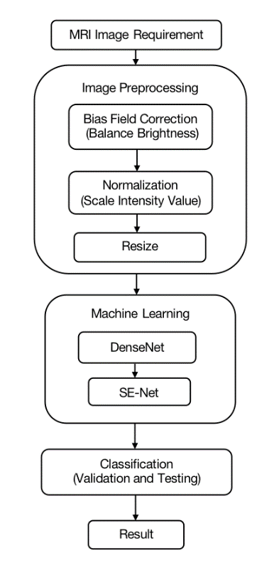
Figure 1. Proposed method for detecting brain tumor in MRI.

3.1. Image preprocessing

The quality of the images input to the machine learning considerably influences the outcome of training the model. The modality of MRI images, the position and orientation of MRI data and the noise are the most important factors that affect the accuracy of image machine learning in the data aspect. Image pre-processing involves normalization, and bias field correction to transform images into comparable datasets.

3.1.1. Bias field correction (BFC) [18]. The proposed method is based on T1-weighted, highlighting the tissues based on water content, and T2-weighted, sensitive to differences in the relaxation time of water molecules in different tissues, MRI data set. In medical imaging, the images produced often have the problem of bias field, which refers to gradual intensity distortion. With varied intensity, it’s hard to perform well on image processing tasks on those images. In order to eliminate this variation, bias field correction is introduced.

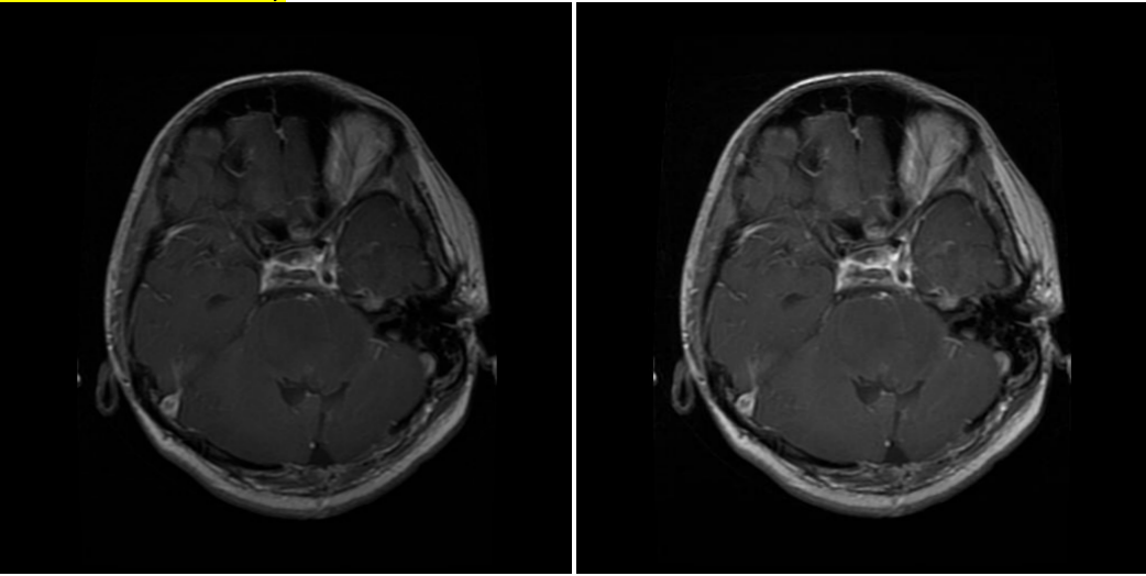
( a ) Glioma MR image before correction. ( b ) Glioma MR image after correction.

Figure 2. (a-b) Images before and after bias field correction.

While BFC focuses on estimating the intensity distortion to eliminate it, the proposed method uses N4 BFC for estimation. Proven for excellent performance on diminishing bias fields, N4 BFC is designed based on the assumption that the corruption of the low-frequency bias field can be represented by the convolution of the intensity histogram by a Gaussian [19]. After deconvolving the intensity histogram by a Gaussian, the function remaps the intensities and then smoothens the result by a B-spline modelling of the bias field itself. In this way, the predicted intensity distortion is removed, and the images are ready to be analysed. Figure 2 shows the effect of Bias Field Correction based on the experiment.

3.1.2. Normalization. The contrast between pixel intensity can largely affect the accuracy of machine learning models on image classification tasks [19]. MR images have variation of intensity. Therefore, it is important to normalize the pixel intensities in images to reduce the contrast between different images before training the model. Min-Max normalisation method is introduced to rescale each pixel’s value to standard range, i.e.

\( {p_{i}}=\frac{{x_{i}}-{x_{min}}}{{x_{max}}{- {x_{min}}}} \) (1)

The pixel (where i = 1,2,3…n in the image) intensity will be scaled to [0, 1] where 0 is the min pixel intensity and 1 is the max pixel intensity in the images.

3.2. Machine learning model

The attention mechanism-based DenseNet model combines DenseNet and SE-Net models. Our model has a squeeze and excitation layer after each Dense transition block in order to reduce the number of calculations which increases with the number of layers. In the dense block, dense connectivity [Equation 2] is used to pass the feature from each layer to the rest of layers [20]. Due to this, the features in the image will be reused and mitigate the gradient loss in the process of machine learning.

\( {x_{l}}=H([{x_{0}},{x_{1}},…,{x_{l-1}}]) \) (2)

While the basic DenseNet model uses the bottleneck layer to decrease the feature outputs, it does not differentiate the significance of each output channel based on their feature importance. To promote network efficiency, the proposed method combines SE-Net with DenseNet. The structure is shown in Figure 3 below.

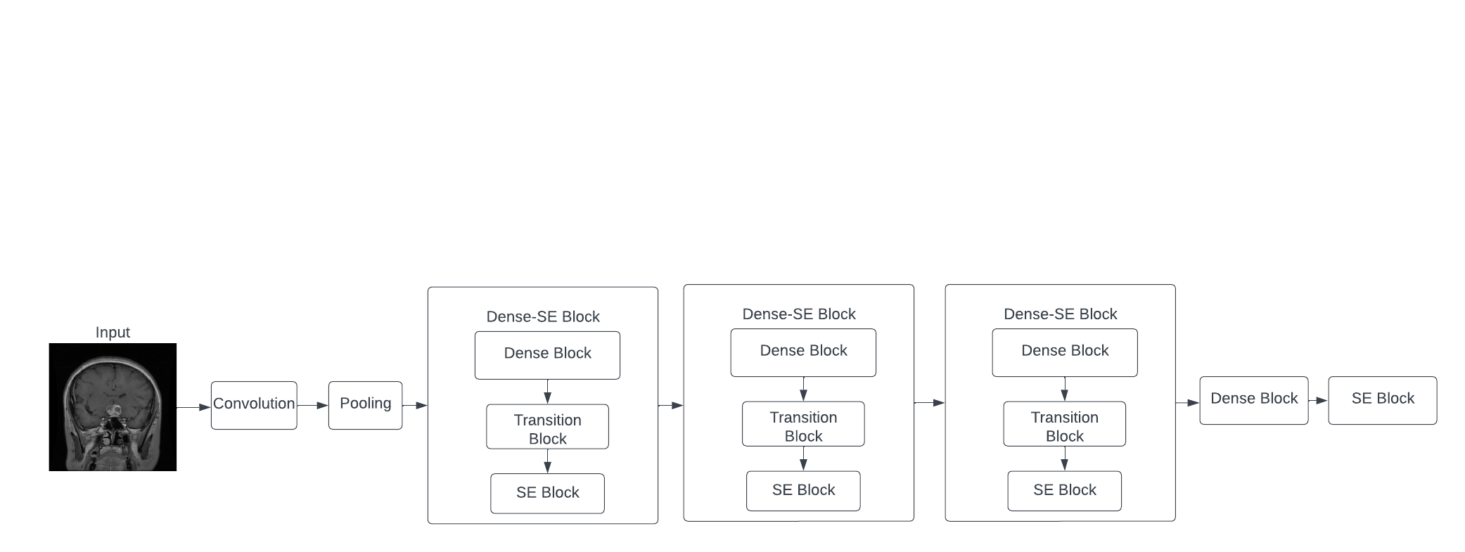
Figure 3. DenseNet based SE-Net model with Dense-SE blocks.

The proposed model first converts the image into comparable data through convolution, and max-pooling is used to down-sample and extract the most significant features. Then 3 Dense-SE block, which contains Dense block and SE block are used, which utilized DenseNet and SE-Net respectively. Finally, one dense block and one SE block define the output and show the classification of the image. The DenseNet and the SE-Net are explained below.

3.2.1. Densely connected convolutional networks (DenseNet). In the CNN model, when the number of layers for the model increases, the model can cope with more complicated data. However, when this number is too large, it may increase the error instead because of vanishing gradients between layers [21]. In MR image classification task, the model needs to have enough depth to analyze the complex information given in the images, so vanishing gradients are inevitable while using CNN models. In order to solve this problem, Dense Convolutional Network (DenseNet) is introduced [22].

Instead of just connecting the consecutive layers, DenseNet has layers that are connected with all previous layers with certain weights to reserve as much information as possible. To achieve this, the activation function, the function to transform input into output, for the model for a certain layer involves the information from all former layers, i.e.

\( {a^{l}}=g({Z^{l}}+\sum _{k=2}^{K}{W^{l-k, l}}∙{a^{l-k}}) \) (3) [23]

where \( {a^{l}} \) is the output of neurons in layer \( l \) , g is the activation function for layer \( l \) , \( {W^{l-k, l}} \) is the weight matrix for neurons between layer \( l-k \) and \( l \) , and \( {Z^{l}}={W^{l-1, l }}∙{a^{l-1}}+{b^{l}} \)

As the features are recalled in each layer, another advantage for using DenseNet is that the features are reinforced for better extraction. Moreover, the required number of parameters is significantly reduced in the DenseNet model. In the context of MRI, the features of different tumors are better extracted for more efficient and accurate classification.

3.2.2. Squeeze and excitation network (SE-Net) [22]. Unlike other classification tasks, MRI images generally have very similar shape and intensity arrangement, which make them hard to be distinguished with each other even manually. To improve the machine’s ability to recognize different images, Squeeze and Excitation Network is introduced into the basic structure of CNN model. While in CNN all the channels have the same weight towards the output, SE-Net utilizes a squeeze operation and an excitation operation to form a content-aware mechanism to weigh each channel adaptively (Figure 4). Using average pooling, the squeeze operation reduces the input features into a single feature vector, which shows the importance of each channel. Through excitation operation, the importance vector acts as the weight for each original channel and the model synthesizes outputs based on the features’ individual importance. Through the use of SE-Net, each feature maps with their significance to better perform image classification.

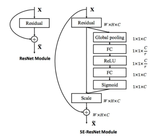
Figure 4. The schema of the original residual module (left) and the SE-ResNet module (right) [22].

4. Experimental results

4.1. Datasets

The MRI dataset used in the experiment contains T1-weighted and T2-weighted images of human brains, from all three anatomical body planes (i.e., axial, coronal, and sagittal) [24]. Out of the original 7022 images, the dataset is divided into three groups: training, testing, and validation, in the approximate ratio of 7:2:1(Figure 5). The images are manually labelled to three types of tumors (i.e., pituitary, meningioma and glioma tumor), or no tumor, with these types of images sharing a similar proportion in all three groups.

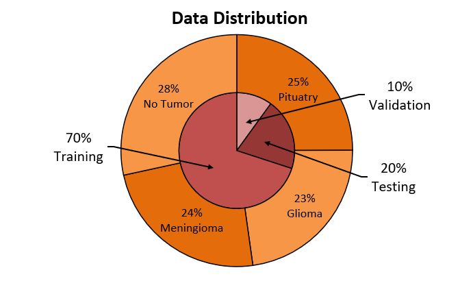
Figure 5. Percentage of data used for each purpose.

The original dataset was cleaned by removing 42 images that had inaccurate classifications of tumor types or undesirable resolutions. The sagittal images are manually axially flipped to face in one direction, which to mitigate the effect of model training. Before the data generating and feeding process, the bias field of each image has corrected by Advanced Normalization Tool (ANTS).

4.2. Experiment setup

The code for this MRI image classification task was developed by Python with major related libraries Tensorflow2.0 and Keras [25]. It is executed with RTX 3080Ti signal channel GPU with 12GB RAM and Intel(R) Xeon(R) 2.50GHz Two cores CPU.

Through trial and error, we decided to train the model over many iterations using batches of size 20, with a reduction of 0.5, as was shown to be optimal for the hardware we used. The initial learning rate is 0.01, which would decay over the training process (et al. it drops to 0.025 when 10 epoch is reached and decreases to 0.001 on 20 epochs). The learning rate decay allows the CNN to learn efficiently in the early stages and slows down as it approaches the point of overfitting to maximize accuracy. The optimizer used is ADAM and categorical crossentropy is used as the loss function in this classification task. The training process took on average approximately 4 minutes per epoch with 30 epochs. To shorten the training time, the early stopping method is implemented so that the training process will be terminated if the performance measured in training loss does not improve in 5 epochs [26]. This mechanism would effectively regulate the training duration and minimize overfitting.

4.3. Result and data analysis

Through the process, the training accuracy would increase to around 99%, at which the curve flattens (Figure 6). Meanwhile, despite greater fluctuations (due to randomly chosen starting points during the gradient descent algorithm), the validation accuracy would also increase until around the end of the 30-epoch time span, at which point the validation accuracy is about 91.32%. At this point, the difference between validation and training accuracy is the smallest. This difference in accuracy as the validation curve flattens is in a fairly decent magnitude, and the difference is minimal at 30 epochs, where the training ends, therefore indicating that overfitting and underfitting are effectively handled.

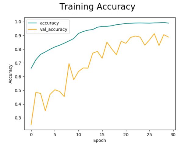
Figure 6. Training accuracy.

The total training time is 120 minutes for 30 epochs. Compared with past research, our model spent much less time on training while providing relatively good performance on brain tumor classification tasks. For example, Wang et al. reported approximately 48 hours of training on a workstation with NVIDIA Tesla V100 GPU with a classification accuracy of 87.21% [27]. Liu et al. reported 70 hours of training on a workstation with 4 NVIDIA Titan X GPUs for segmentation and classification tasks in total with a classification accuracy of 94.16%, compared with 2 hours of training with 91.32% accuracy in our model [28].

Moreover, according to F1 score as calculated below, our proposed method shows competitive performance under a limited amount of data [29]. The details about the evaluation methods are shown below:

\( Precision=TP/(TP+FP) \) (4)

\( Recall=TP/(TP+FN) \) (5)

\( f1 score=\frac{2×Precision×Recall}{Precision+Recall}=\frac{TP}{TP+\frac{1}{2}(FP+FN)} \) (6)

Where TP, TN, FP, and FN refer to true positive, true negative, false positive, and false negative. While considering each type of tumor, the positive label is given to exactly this type of tumor and the negative label is given to all other types. According to the confusion matrix (Figure 7), the Precision, recall, and f1 score can be calculated as shown in Table 1.

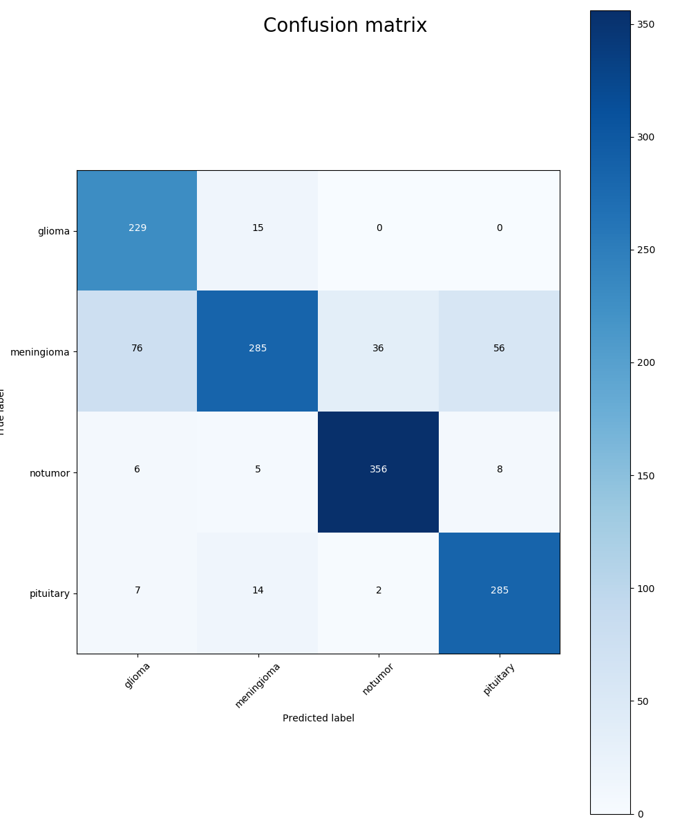
Figure 7. Confusion matrix: the x-axis is the predicted label and the y-axis is the true label.

Table 1. F1 score calculated.

As is observed in the table, our model is relatively weak on identifying meningioma tumors. If meningioma is taken from the data, the f1 scores of glioma, pituitary, and no tumor are 0.95, 0.97, and 0.96 with an average f1 score 0.9607, which proves excellent performance in identifying glioma, pituitary, or no tumor images.

5. Conclusion

In this paper, we proposed an advanced machine learning method consisting of Densely Connected Convolutional Networks and Squeeze and Excitation Networks with proven suitability for brain tumor classification tasks. With a limited amount of pre-processed T1-weighted and T2-weighted brain MRI images, our proposed method is designed to be simple and less time-consuming while indicating competitive performance. As evaluated by f1 score, the proposed model shows excellent performance in classifying all the tumor types except a mild defect in classifying Meningioma. It is worth trying to feed the model with a larger amount of data to improve its performance. Moreover, the model can be pre-trained on ImageNet for transfer learning. The model can also be implemented on other MR images such as cardiac MRI images to extend its application.

References

[1]. Chavan, N. V., Jadhav, B. D., & Patil, P. M. (2015). Detection and classification of brain tumors. International Journal of Computer Applications, 112(8).
[2]. Mayo Foundation for Medical Education and Research. (2023, February 10). Brain Tumor. Mayo Clinic. Retrieved February 14, 2023, from https://www.mayoclinic.org/diseases-conditions/brain-tumor/symptoms-causes/syc-20350084。
[3]. Rehman, A., Naz, S., Razzak, M. I., Akram, F., & Imran, M. (2020). A deep learning-based framework for automatic brain tumors classification using transfer learning. Circuits, Systems, and Signal Processing, 39, 757-775.
[4]. Brain MRI: What it is, purpose, procedure & results. Cleveland Clinic. (2022, September 5). Retrieved February 15, 2023, from https://my.clevelandclinic.org/health/diagnostics/22966-brain-mri.
[5]. Radiological Society of North America (RSNA) and American College of Radiology (ACR). (2022, April 15). Brain tumors. Radiologyinfo.org. Retrieved February 15, 2023, from https://www.radiologyinfo.org/en/info/braintumor.
[6]. Sharma, K., Kaur, A., & Gujral, S. (2014). Brain tumor detection based on machine learning algorithms. International Journal of Computer Applications, 103(1).
[7]. Tang, J., Alelyani, S., & Liu, H. (2014). Feature selection for classification: A review. *Data classification: Algorithms and applications*, 37.
[8]. Garg, M., & Dhiman, G. (2021). A novel content-based image retrieval approach for classification using GLCM features and texture fused LBP variants. *Neural Computing and Applications*, *33*, 1311-1328.
[9]. Jiang, J., Wu, Y., Huang, M., Yang, W., Chen, W., & Feng, Q. (2013). 3D brain tumor segmentation in multimodal MR images based on learning population-and patient-specific feature sets. *Computerized Medical Imaging and Graphics*, *37*(7-8), 512-521.
[10]. Cheng, J., Yang, W., Huang, M., Huang, W., Jiang, J., Zhou, Y., ... & Chen, W. (2016). Retrieval of brain tumors by adaptive spatial pooling and fisher vector representation. *PloS one*, *11*(6), e0157112.
[11]. Zhi, L. J., Zhang, S. M., Zhao, D. Z., Zhao, H., & Lin, S. K. (2009, October). Medical image retrieval using SIFT feature. In *2009 2nd International Congress on Image and Signal Processing* (pp. 1-4). IEEE.
[12]. Cui, S., Jiang, H., Wang, Z., & Shen, C. (2017, June). Application of neural network based on SIFT local feature extraction in medical image classification. In *2017 2nd International Conference on Image, Vision and Computing (ICIVC)* (pp. 92-97). IEEE.
[13]. Saxena, S., & Gyanchandani, M. (2020). Machine learning methods for computer-aided breast cancer diagnosis using histopathology: a narrative review. *Journal of medical imaging and radiation sciences*, *51*(1), 182-193.
[14]. Razzak, M. I., Naz, S., & Zaib, A. (2018). Deep learning for medical image processing: Overview, challenges and the future. *Classification in BioApps: Automation of Decision Making*, 323-350.
[15]. Hashemzehi, R., Mahdavi, S. J. S., Kheirabadi, M., & Kamel, S. R. (2020). Detection of brain tumors from MRI images base on deep learning using hybrid model CNN and NADE. *biocybernetics and biomedical engineering*, *40*(3), 1225-1232.
[16]. Kaldera, H. N. T. K., Gunasekara, S. R., & Dissanayake, M. B. (2019, March). Brain tumor classification and segmentation using faster R-CNN. In 2019 Advances in Science and Engineering Technology International Conferences (ASET) (pp. 1-6). IEEE.
[17]. Sahaai, M. B., Jothilakshmi, G. R., Ravikumar, D., Prasath, R., & Singh, S. (2022, May). ResNet-50 based deep neural network using transfer learning for brain tumor classification. In AIP Conference Proceedings (Vol. 2463, No. 1, p. 020014). AIP Publishing LLC.
[18]. Karim, F., & Islam, M. T. (2018). An overview of bias field correction in MRI. Journal of Health and Medical Informatics, 9(2), 1000302.
[19]. Khan Swati ZN, Zhao Q, Kabir M, Ali F, Ali Z, Ahmed S, Lu J, Brain tumor classification for MR images using transfer learning and fine-tuning, Computerized Medical Imaging and Graphics (2019), https://doi.org/10.1016/j.compmedimag.2019.05.001
[20]. Huang, G., Liu, Z., Van Der Maaten, L., & Weinberger, K. Q. (2018). Densely connected convolutional networks. In Proceedings of the IEEE conference on computer vision and pattern recognition (pp. 4700-4708).
[21]. Tustison, N. J., Avants, B. B., Cook, P. A., Zheng, Y., Egan, A., Yushkevich, P. A., & Gee, J. C. (2010). N4ITK: improved N3 bias correction. IEEE transactions on medical imaging, 29(6), 1310–1320. https://doi.org/10.1109/TMI.2010.2046908
[22]. Hu, J., Shen, L., & Sun, G. (2018). Squeeze-and-excitation networks. In Proceedings of the IEEE conference on computer vision and pattern recognition (pp. 7132-7141).
[23]. Huang, G., Gao, L., Liu, Z., Van Der Maaten, L., & Weinberger, K. Q. (2017). Densely Connected Convolutional Networks. In 2017 IEEE Conference on Computer Vision and Pattern Recognition (CVPR) (pp. 2261-2269). Honolulu, HI: IEEE. doi:10.1109/CVPR.2017.243
[24]. Nickparvar, M. (2021, September 24). Brain tumor MRI dataset. Kaggle. Retrieved March 23, 2023, from https://www.kaggle.com/datasets/masoudnickparvar/brain-tumor-mri-dataset
[25]. Abadi, M., Agarwal, A., Barham, P., Brevdo, E., Chen, Z., Citro, C., ... & Zheng, X. (2016). Tensorflow: Large-scale machine learning on heterogeneous distributed systems. arXiv preprint arXiv:1603.04467.
[26]. Brownlee, J. (2018). Early stopping to avoid overfitting in neural networks. Machine Learning Mastery. https://machinelearningmastery.com/how-to-stop-training-deep-neural-networks-at-the-right-time-using-early-stopping/
[27]. Wang, G., Li, W., Aertsen, M., & De Vleeschouwer, S. (2020). A novel deep learning-based method for predicting IDH genotype in brain gliomas from preoperative MRI. European Radiology, 30(7), 4014-4023. doi: 10.1007/s00330-020-06733-w.
[28]. Liu, S., Wang, X., Liu, S., Liu, X., Zeng, N., & Zhang, X. (2020). Multi-task learning based on 3D residual convolutional neural network for brain tumor segmentation and classification. Neurocomputing, 404, 1-9. doi: 10.1016/j.neucom.2020.05.065.
[29]. Van Rijsbergen, C. J. (1979). Information Retrieval. Butterworths.
Cite this article
Tang,M.;Gao,L.;Bian,Y.;Xiang,S.;Zhang,K. (2023). Brain tumor MRI images classification based on machine learning. Applied and Computational Engineering,29,19-29.
Data availability
The datasets used and/or analyzed during the current study will be available from the authors upon reasonable request.
Disclaimer/Publisher's Note
The statements, opinions and data contained in all publications are solely those of the individual author(s) and contributor(s) and not of EWA Publishing and/or the editor(s). EWA Publishing and/or the editor(s) disclaim responsibility for any injury to people or property resulting from any ideas, methods, instructions or products referred to in the content.
About volume
Volume title: Proceedings of the 5th International Conference on Computing and Data Science
© 2024 by the author(s). Licensee EWA Publishing, Oxford, UK. This article is an open access article distributed under the terms and
conditions of the Creative Commons Attribution (CC BY) license. Authors who
publish this series agree to the following terms:
1. Authors retain copyright and grant the series right of first publication with the work simultaneously licensed under a Creative Commons
Attribution License that allows others to share the work with an acknowledgment of the work's authorship and initial publication in this
series.
2. Authors are able to enter into separate, additional contractual arrangements for the non-exclusive distribution of the series's published
version of the work (e.g., post it to an institutional repository or publish it in a book), with an acknowledgment of its initial
publication in this series.
3. Authors are permitted and encouraged to post their work online (e.g., in institutional repositories or on their website) prior to and
during the submission process, as it can lead to productive exchanges, as well as earlier and greater citation of published work (See
Open access policy for details).