1. Introduction

The development of green finance in China has displayed a consistent upward trajectory. Nevertheless, this advancement faces obstacles attributable to factors such as inadequate institutional mechanisms and disparities in financial resource allocations. Consequently, the variances in economic development among different regions have led to an imbalance in the coordinated progress of green finance [1-2]. Research has indicated that the implementation of relevant policies has contributed to a regional inclination toward balanced development in China’s green finance landscape [3]. During the 75th United Nations General Assembly in 2020, President Xi Jinping made a global commitment, stating that China would strive to achieve a peak in carbon dioxide emissions by 2030 and endeavor to attain carbon neutrality by 2060. Green finance serves as a framework grounded in the principles of promoting green transformation and low carbon finance. It facilitates the flow of financial resources toward projects related to green and low-carbon initiatives within cities. Green finance primarily targets economic activities that encompass environmental improvement, climate change response, and efficient resource utilization in urban areas. This approach encourages enterprises to engage in energy-saving, environmentally friendly, and green and low-carbon practices, ultimately enhancing the quality of urban development. This is achieved through the establishment of industrial green credit channels and the alleviation of financing constraints associated with green transformation [4].

When studying the impact of green finance on urban high-quality development, scholars predominantly adopt an economic perspective to explore the relationship [5-9]. However, there is a lack of consistent research focus on the G-FINANCING INDEX, which is a comprehensive indicator constructed from multiple dimensions such as green carbon finance, green investment, and green bonds. Currently, research efforts are increasingly directed towards understanding this index and its implications [10-13]. The factors influencing green finance can be categorized into endogenous and exogenous factors. Research on exogenous factors primarily focuses on the regional and urban perspectives, analyzing the heterogeneous impact of green finance on the high-quality development of cities. The aim is to provide empirical references for the integration of green finance with the real economy and facilitate the high-quality development of cities [14]. The current mainstream research method combines the dynamic spatial Durbin model with spatial correlation analysis tools. This approach effectively constructs a spatial matrix and tests the spatial correlation and spillover effects of green finance [15]. When it comes to endogenous factors, green finance possesses financial characteristics that attract a significant number of low-carbon industries. By relaxing the financing requirements for green and low-carbon industries, green finance strengthens the connection between financial institutions and industries within cities. This, in turn, reduces transaction costs for industries and plays a pivotal role in driving the collaborative development of upstream and downstream industries within a city [16]. However, existing studies mainly describe relationships within global or local regions, leaving ample room for research on the interplay between the development of green finance in different regions or provinces [17].

In light of these considerations, this research adopts a comprehensive approach. It constructs a holistic index system by integrating various economic elements, including carbon finance, green investment, green insurance, and green bonds. The VIKOR algorithm is employed to conduct a comprehensive assessment of the G-FINANCING index at the provincial level in China. This evaluation serves as the basis for organizing the spatial and temporal distribution patterns of green financial development. Moreover, by establishing a Markov spatial transfer matrix, the study analyzes the migration and discrete trends of hotspot areas. Additionally, the future development patterns of green finance in China’s three major economic belts are predicted using the machine learning algorithm ADABOOST. This approach serves as an effective strategy for bridging the regional gap in the level of green finance. It facilitates the spatially coordinated development of the green finance sector, offering a robust theoretical foundation for further narrowing the regional disparity in green finance.

2. Modelling

2.1. The VIKOR Method

The VIKOR method, an applicable technique used in Multiple Criteria Decision Making (MCDM), has been developed specifically to address discrete decision-making problems. It effectively handles criteria that are non-commensurable or have different units, making it suitable for situations where comparisons are challenging. Its primary objective is to rank and select alternatives by providing a compromise solution that accommodates conflicting criteria faced by decision makers. To achieve this, a multi-criteria measure for compromise ranking is derived from the LP-metric. This measure serves as an aggregating function within a compromise programming method. Thus, the VIKOR method serves as a valuable tool to aid decision makers in selecting the optimal solution, as it effectively considers and reconciles conflicts inherent in decision-making scenarios.

To perform the compromise ranking of alternatives based on their evaluations according to each criterion, we utilize the measure of closeness to the ideal alternative. The set of alternatives is denoted as A1, A2, ..., Am, where each alternative Ai is assigned a rating for the jth aspect represented by \( {f_{ij}} \) indicating the value of the jth criterion function for alternative Ai. The total number of criteria is denoted as n. The development of the VIKOR method starts with formulating the LP-metric in the following manner:

\( \begin{array}{c} {L_{pi}}={\lbrace \sum _{j=1}^{n}[\frac{f_{j}^{*}-{f_{ij}}}{(f_{j}^{*}-f_{j}^{-}){]^{p}}}\rbrace ^{\frac{1}{p}}}1⩽p⩽∞; \\ i=1,2,…,m. \end{array} \) (1)

To formulate the ranking measure in the VIKOR method, two key indicators, min Si and min Ri, are utilized. The solution attained by minimizing Si represents the maximum group utility, following the principle of “majority” rule. On the other hand, minimizing Ri in the VIKOR method yields a solution that corresponds to the minimum individual regret of the “opponent”. The compromise ranking algorithm in the VIKOR method entails the following steps:

(a) The first step in the VIKOR method is to identify the best \( f_{j}^{*} \) and the worst \( f_{j}^{-} \) values for each criterion function \( j = 1, 2, …, n \) . If the jth function denotes a benefit, then it follows that:

\( f_{j}^{*}=\underset{i}{max{{f_{ij}}}},f_{j}^{-}=\underset{i}{min{{f_{ij}}}} \) (2)

(b) Compute the values \( {S_{i}} \) and \( {R_{i}} \) ; i = 1, 2, …, m, by these relations:

\( \begin{matrix} & {S_{i}}=\sum _{j=1}^{n}\frac{{w_{j}}(f_{j}^{*}-{f_{ij}})}{f_{j}^{*}-f_{j}^{-}}, \\ & \\ & {R_{i}}=\frac{\underset{j}{max{{w_{j}}(f_{j}^{*}-{f_{ij}})}}}{f_{j}^{*}-f_{j}^{-}}, \\ \end{matrix} \) (3)

This is determined by assigning weights \( {w_{j}} \) to the criteria, which reflect their respective levels of importance within the analysis.

(c) The values \( {Q_{i}} \) ; \( i = 1, 2, …, m, \) can be calculated using the following equation:

\( \begin{matrix} & \\ & \\ \end{matrix}{Q_{i}}=\frac{v({S_{i}}-{S^{*}})}{{S^{-}}-{S^{*}}}+\frac{(1-v)({R_{i}}-{R^{*}})}{{R^{-}}-{R^{*}}} \) (4)

Where \( {S^{*}}=\underset{i}{min⁡}{S_{i}},{S^{-}}=\underset{i}{max⁡}{S_{i}} \)

\( {R^{*}}=\underset{i}{min⁡}{R_{i}},{R^{-}}=\underset{i}{max⁡}{R_{i}} \)

Let us introduce the weight, denoted as \( v \) , for the strategy of “the majority of criteria” or “the maximum group utility”. In this case, let’s assume that \( v=0.5 \)

(d) Sort the alternatives in descending order based on the values of S, R, and Q. This will generate three separate ranking lists.

(e) If the following two conditions are met, the alternative A’ will be proposed as the compromise solution, as it ranks highest according to the Q (Minimum) measure:

1. Acceptable advantage: \( Q({A^{ \prime \prime }})-Q({A^{ \prime }})⩾DQ \)

The alternative \( {A^{ \prime \prime }} \) refers to the option ranked second in the Q-based ranking list. If this alternative meets the following two conditions: \( DQ=1/(m-1) \) ; \( m \) represents the total number of alternatives available for evaluation.

2. Acceptable stability in decision making:

For alternative A’, it is crucial that it holds the highest ranking in terms of S or/and R. This compromise solution ensures stability in the decision-making process, which can be achieved either through “voting by majority rule” (when \( v \gt 0.5 \) is needed) or by striving for a consensus among the decision-makers. \( v=0.5 \) , or “with veto” ( \( v \lt 0.5 \) ). In this context, the weight v corresponds to the decision-making strategy of “the majority of criteria” or “the maximum group utility”. If either of the conditions mentioned earlier is not met, a set of compromise solutions will be suggested.

The alternative that achieves the lowest value of Q is considered the best alternative in terms of the Q ranking. The primary outcome of the ranking process is the compromise ranking list of alternatives, which identifies the compromise solution along with its corresponding “advantage rate”.

2.2. Markov Chain

For a discrete time Markov chain, the probabilities of transitions satisfy a fundamental relation called Chapman-Kolmogorov equation.

\( \begin{matrix} & {P_{i,j}}(0,t+s)=P(X(t+s)=\frac{j}{X(0)}=i) & \\ & =\sum _{f}P(X(t+s)=j,X(t)=\frac{f}{X(0)}=i) & \\ & =\sum _{f}P(X(t+s)=j,X(t)=\frac{f}{X(0)}=i)P(X(t)=\frac{f}{X(0)}=i) & \\ & =\sum _{f}P(X(t+s)=\frac{j}{X(t)}=f)P(X(t)=\frac{f}{X(0)}=i) & \\ & =\sum _{f}{P_{i,f}}(0,t){P_{f,j}}(t,t+s). & \\ \end{matrix} \) (5)

In the context of a Markov chain, a probability law π on the state space is referred to as stationary if it remains unchanged when the chain transitions from one state to another.

Let’s denote π(t) as a probability vector associated with the set of states E in the given Markov chain. This vector is defined by the equation:

\( п:{π_{i}}(t)=P(X(t)=i) \) (6)

\( π(t)=({π_{1}}(t),{π_{2}}(t),…{π_{m}}(t)) \) (7)

The sum of probabilities in this vector can be expressed as: \( ∑π(t)=1 \) is equal to 1. The probability vector is referred to as the “stable law” of the Markov chain if it satisfies the condition: \( π(t)= π(t)P \) .

2.3. Kernel Density Estimation

Kernel density estimation is a method used to estimate the probability density of a random variable. It achieves this by utilizing a smooth and continuous density curve. One of the strengths of this approach is its robustness, as it is not overly reliant on specific model assumptions or parameter settings. Consequently, the estimation results tend to be reliable and less affected by those factors. In this research, the G-FINANCING INDEX is represented by several characteristics derived from the kernel density curve. These characteristics include the vertical position of the distribution, the height and width of the peaks, the number of peaks, and the distribution extensibility. Additionally, these characteristics also reflect the clustering patterns, polarization trends, and degree of variation among provinces. \( f(a) \) is the probability density of the density function of the random variable A at the point a, \( n \) is the number of provinces, \( h \) is the bandwidth, and \( K(·) \) is the Gaussian kernel function.

\( f(a)=(1/nh)\sum _{i=1}^{n}K[\frac{{A_{i}}-a}{h}] \) (8)

\( K(a)=(\frac{1}{\sqrt[]{2π}})exp{(-\frac{{a^{2}}}{2})} \) (9)

2.4. AdaBoost

AdaBoost, also known as “Adaptive Boosting,” is a machine learning technique that exhibits sensitivity to noisy and abnormal data. Nevertheless, compared to various other learning algorithms, the AdaBoost method demonstrates relatively lower susceptibility to overfitting in specific problem domains.

Denote by \( xi, \) and \( yi \) the sample points of the original sample set D and their class labels. Denote by \( Wk(i) \) the weight distribution of all samples at the kth iteration.

(1) During the initialization stage, the training set serves as the input, encompassing the necessary parameters. \( D=\lbrace x1,y1,...,xn,yn\rbrace \) , The initialization process involves assigning the maximum number of cycles kmax and the sampling weights \( Wk(i)=1/n \) based on the training set. The iteration counter k is set to 0 initially and subsequently incremented by 1 in each iteration.

(2) The weak learner Ck is trained by utilizing the sampling weights \( Wk(i) \) during the training process.

(3) The training results of the weak learner Ck are evaluated, and subsequently, they are recorded into the error matrix \( {E_{k}} \) .

\( {α_{k}}←\frac{1}{2}ln{\frac{1-{E_{k}}}{{E_{k}}}} \) (10)

\( {W_{k+1}}(i)←\frac{{W_{k}}(i)}{{Z_{k}}}×\lbrace \begin{array}{c} {e^{-{α_{k}}}},if {h_{k}}({x^{i}})={y_{i}}, \\ {e^{{α_{k}}}},if {h_{k}}({x^{i}})≠{y_{i}} \end{array} \) (11)

Stop training when \( k=kmax \)

Return results \( Ck \) and \( {α_{k}} \) , \( k=1, ... , kmax (overall with weights) \)

3. Temporal Evolutionary Characteristics of Green Finance Development

During China’s seventh five-year plan period, some cities were divided into three economic zones: eastern, central and western. This article uses selected cities as the research subjects. Overall, China’s G-FINANCING INDEX shows fluctuating growth during the sample period. World Bank World Development Indicators 2010 pointed out that the energy consumption of China’s industrial sector is responsible for approximately 70 percent of the total energy consumption. Moreover, the resulting carbon emissions from this sector account for around 85 percent of the total emissions. These figures indicate that there is significant potential for the advancement of green finance in China. In 2016, China, as the rotating president of the G20 Summit, incorporated green finance into the core issues of the meeting and set up the G20 Green Finance Study Group [4]. Seven Ministries and Commissions jointly issued “Guiding Opinions on Building a Green Financial System”, which clarified the development direction and target tasks of green finance, under the guidance of the opinions, various regions and industries actively build a green financial system, and explore the effective green financial development model, but the early stage of the release has not yet formed a unified and standardised paradigm for the development of green finance, and in the process, due to the inevitable all-financial resource mismatches and efficiency losses In 2018, the Green Finance Standard Working Group was established, which promoted the rapid improvement of the green finance level by constructing a perfect cross-field, market-oriented green finance standard system embedded in the whole business process of financial institutions. From 2018 to 2021, the China Green Bond Support Project Catalogue (2021 Edition), Environmental Information Disclosure Guidelines for Financial Institutions and Environmental Equity Financing Instruments were formally released; providing a strong impetus to the construction and sustainable development of the domestic green financial market environment.

For the different sub-regions, the G-FINANCING INDEX in the three major economic belts exhibits a fluctuating upward trend. Notably, the level of green finance in the eastern region consistently surpasses the national average. The eastern region boasts a robust economic foundation and a stable financial system. In comparison to the central, western, and northeastern regions, its favorable conditions for the advancement of green finance are evident. Furthermore, the eastern region places a higher importance on environmental protection policies and has implemented them more vigorously. The concept of green development has been widely adopted and disseminated in this region. The ongoing green transformation of polluting industries has generated a substantial demand for green funds, consequently fostering the growth of green finance within the eastern region. Additionally, the level of green finance in the central region has exhibited a consistent upward trend, surpassing the national average in 2016. It is found that during the period of 2014-2016, the scale of credit for high energy-consuming enterprises in the central region was significantly reduced and accompanied by a significant increase in GREEN INVESTMENT, which may be one of the reasons for the climb in the level of CARBON FINANCE in the central region. The gap between the G-FINANCING INDEX in the western and northeastern regions is relatively small, showing a staggered upward trend, and both are lower than the national average level. Western and northeastern industrial volume is too large and the industrial structure is relatively single, the resource-dependent development mode to a certain extent caused by the mismatch of financial resources. Moreover, the development of green finance is hindered by factors such as the inactivity of the financial market and the absence of incentives for the implementation of green finance policies.

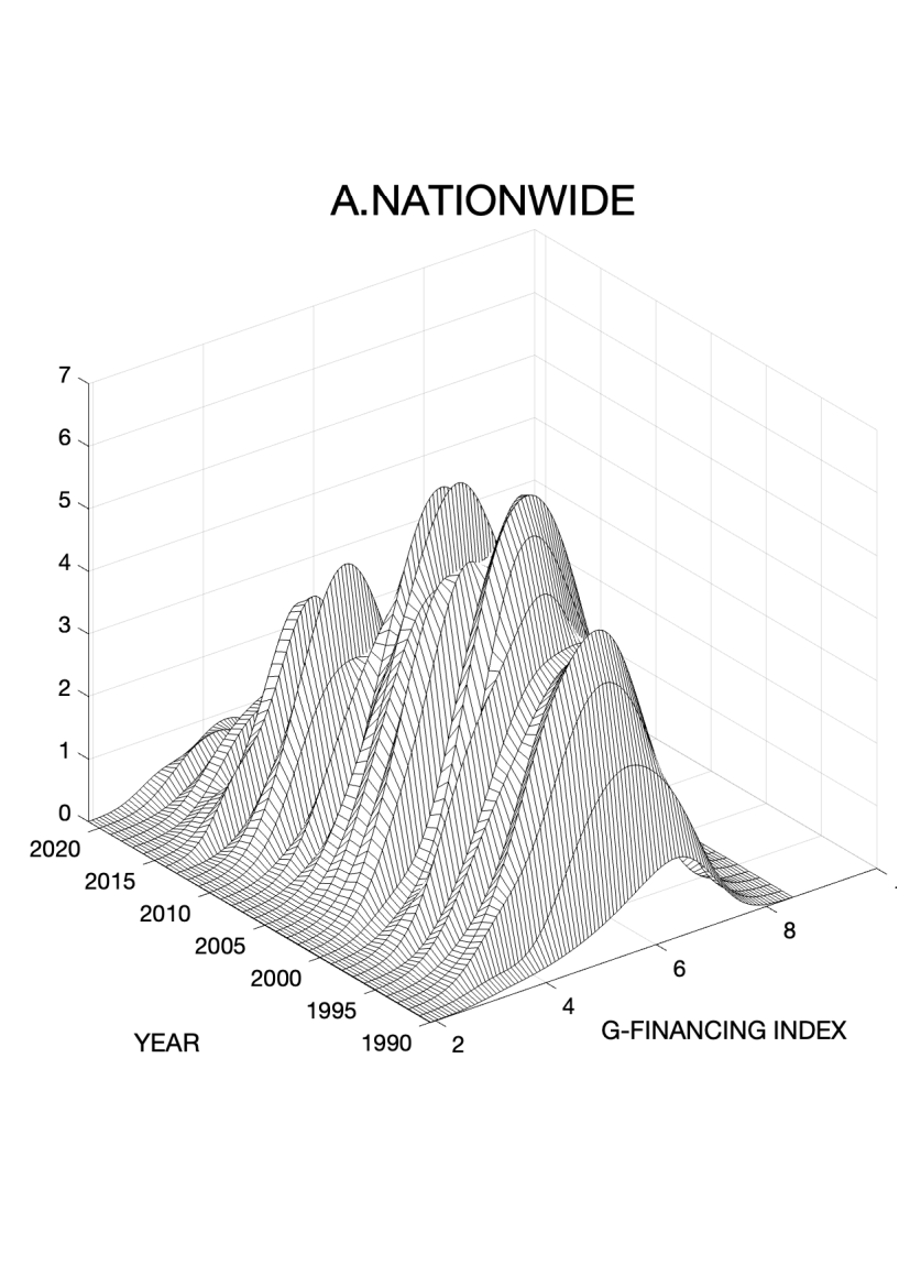
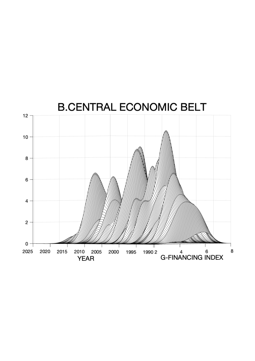
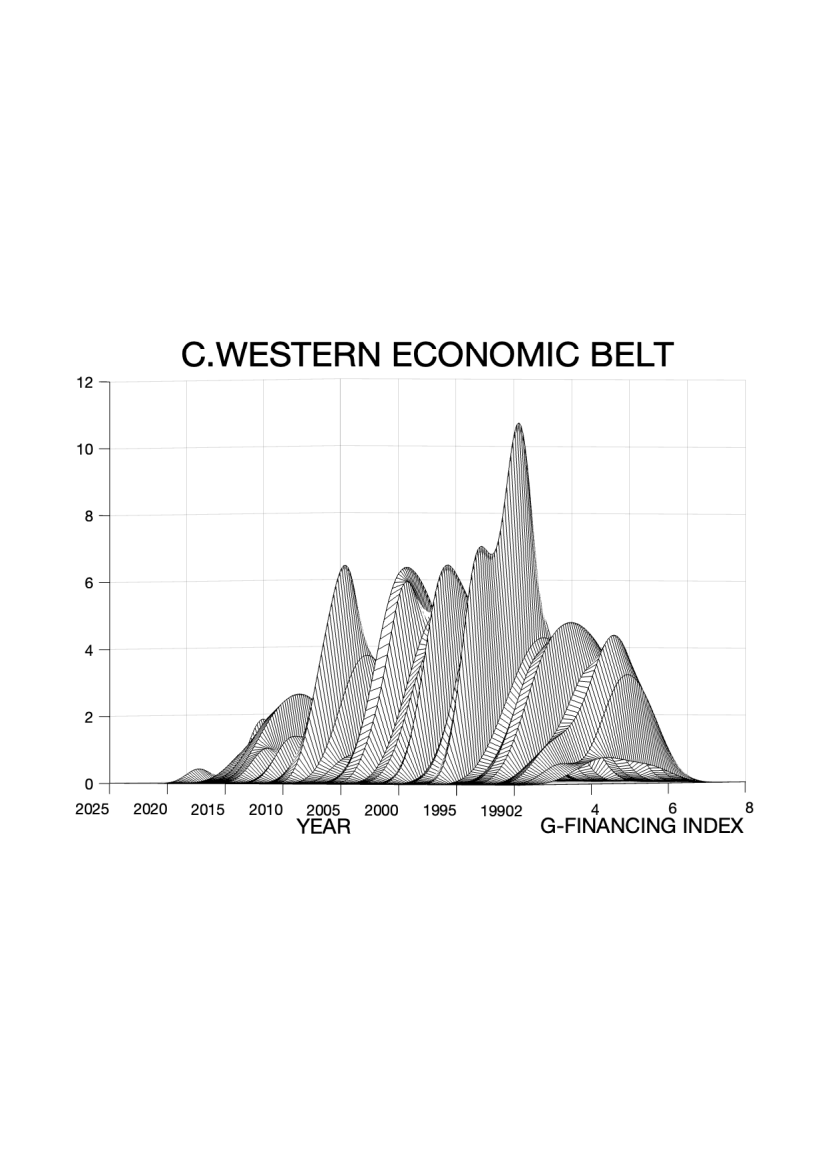
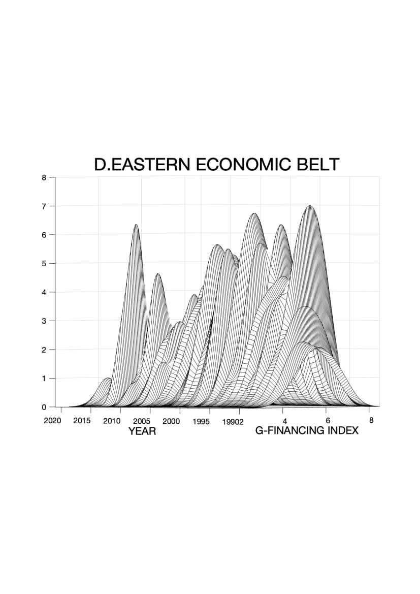
Figure 1: Dynamic Kernel Density Graph of Green Finance.

Throughout the study period, the central economic belt consistently exhibited strong development momentum. At the outset of the research, the kernel density curve in the central region displayed a noticeable trend of rightward concentration. In comparison to other regions, it demonstrated both favorable and unfavorable performance.After 2020, the distribution of the kernel density curve expanded to some extent, indicating that the initial development of green finance in the region exhibited a certain scale effect. Although the development trend decelerated comparatively, there was a positive transfer of development momentum among cities. In the western economic zone, the right side of the kernel density curve corresponds to the higher end of the density distribution. The right side of the curve of nuclear density in the western economic belt has a clear trailing trend, and the overall degree of enhancement is high. At the end of the last century, the overall development of the western region is limited, the kernel density curve aggregation degree is high and the bandwidth is limited, which can be seen in the western city G-FINANCING INDEX development situation is low, and the overall aggregation of G-FINANCING INDEX of the city group is about 4.5 points. After 2000, the city group in the region gets rid of the decadence, and the overall performance of the multi-peak form, which indicates that there is a phenomenon of multi-polar polarisation among the city group, and some of the cities begin to move towards the high level of development of the city excessively, and green finance develops vigorously within the city clusters.

Unlike other regions, the kernel density map of the eastern economic belt shows the morphological characteristics from sharp to flat, and the flat and wide kernel density curve reflects the development characteristics of the provinces in the region with a large degree of difference. With the continuous development of green finance in the region, the degree of freedom of financial policies and measures in each city has been increasing, the kernel density curve has changed from a single sharp peak to multiple fronts, and the driving force of green finance has gradually slowed down after reaching a peak in 2015, with the city cluster as a whole showing very high development momentum.

4. Spatial Evolution Characteristics of Green Finance

To comprehensively analyze the spatiotemporal evolution patterns of the G-FINANCING INDEX in Chinese cities, we construct both a traditional Markov transfer probability matrix and a spatial-based Markov transfer probability matrix. The G-FINANCING INDEX is classified into four states: low-low, low-high, high-low, and high-high, labeled as k = 1, 2, 3, and 4, respectively. A transfer from low values to high values is considered an upward transfer, while a transfer from high values to low values is considered a downward transfer. This framework allows us to capture the movement and transitions between different value levels of the G-FINANCING INDEX over time and space.

Presented in the subsequent table is the traditional Markov transfer probability matrix for urban G-FINANCING INDEX types across mainland China spanning from 1990 to 2021. Based on the calculation results, the following observations can be made:(i) The probability values associated with the diagonal line consistently surpass those linked to the non-diagonal line. This implies that the transfer of urban G-FINANCING INDEX types in China demonstrates stability, with a higher chance of maintaining the original state. (ii)A phenomenon known as “club convergence” is observed within the G-FINANCING INDEX of Chinese cities. Low and high G-FINANCING INDEX types have the highest probabilities of sustaining their corresponding state in the subsequent stage, standing at 53.03% and 58.54%, respectively. (iii)Transitions between different G-FINANCING INDEX types in consecutive years occur relatively smoothly, and no “leapfrog” development is evident.

Table 1: Spatial Markov Matrix.

To incorporate spatial considerations into the traditional Markov chain transfer probability matrix, we construct the spatial Markov transfer probability matrix. This matrix allows us to investigate how neighborhood characteristics influence the transfer of the urban G-FINANCING INDEX. Through comparing and analyzing the transfer probabilities of the urban G-FINANCING INDEX in various neighborhood backgrounds, we can explore the impact of the neighboring environment. Presented below is the spatial Markov transfer probability matrix for the different types of G-FINANCING INDEX in Chinese cities from 1990 to 2021. Based on the calculated results, the following deductions can be made: (i)Geographic background plays a vital role in the transfer process of G-FINANCING INDEX in Chinese cities. The transfer probability of the G-FINANCING INDEX varies significantly under different geographical backgrounds when compared to the traditional Markov transfer probability matrix. (ii)The G-FINANCING INDEX of cities exhibits synergy with the regional G-FINANCING INDEX type. When the neighborhood type is 1, the number of cities with a low G-FINANCING INDEX during time period t is notably higher than cities of other types. Similarly, when the neighborhood type is 4, the number of cities with a high G-FINANCING INDEX during time period t is significantly greater compared to cities of other types. (iii)Cities have convergence with the economic environment where they are located, and the probability of the type of G-FINANCING INDEX of the city shifting downward increases when the city is in the region with low G-FINANCING INDEX, and the probability of the type of G-FINANCING INDEX of the city shifting upward will increase when the city is in the region with high G-FINANCING INDEX. The spatial Markov transfer probability matrix provides an explanation for the phenomenon of “club convergence” in the spatial dimension.

Table 2: Spatial Lagged Markov Matrix.

5. Forecasts of the Volume of Green Finance

5.1. Forecast of Time Evolution of Green Finance Development

According to the theory of economic growth, the economic activity of a region is the result of a combination of factors such as capital, market, technology and policy. During the study period, economic activity indicators such as CARBON FINANCE, GREEN CREDIT, GREEN SECURITIES, GREEN INSURANCE and GREEN INVESTMENT interacted with each other to form a regional economic development pattern in a geographical context. It is expected that in the future, under the conditions of marketisation and open economy, the free flow of all financial factors under the unified market will allow cities within the economic belt to learn from the advanced technologies of other regions, especially neighbouring regions, and the diminishing marginal utility of policy innovation will prompt intergovernmental learning and imitation of relatively well-developed financial indicators such as GREEN SECURITIES and GREEN INSURANCE.

During the next five years, it is expected that the share of GREEN SECURITIES and GREEN INSURANCE in the industry will reach 0.16 and 0.10, respectively, and the share of the two will rise by 45.12 per cent and 45.82 per cent, respectively, during the twenty-year period. In addition, it is important to consider the spatial spillover effect of economic activities. As the region’s economic development model evolves in synergy with advancements in information technology and continuous improvements in regional infrastructure, the cost of inter-regional flow of financial factors is expected to decrease. This, in turn, will facilitate the free flow of inter-regional financial factors, thereby amplifying the spatial spillover effect of economic activities. During the next five years, the share of Carbon Finance and GREEN INVESTMENT in the industry will reach 0.05 and 0.02 respectively, and the share of the two will rise by 45.12% and 45.82% respectively during the twenty years.

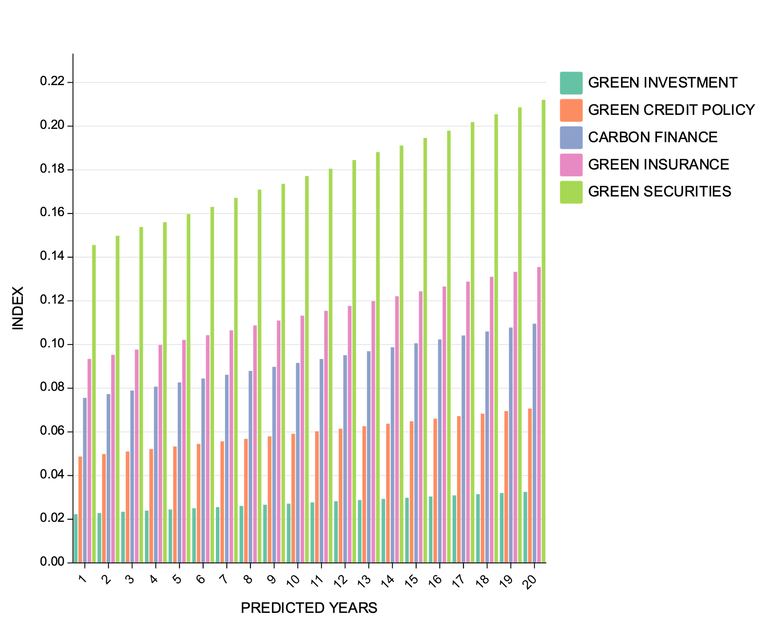
Figure 2: Green Finance Index Prediction Based on Adaboost Method.

5.2. Prediction of the Spatial Evolution of Green Financial Development

The limiting distribution of Markov transfer probability is the distribution under the various types of transfers reaching an equilibrium state, and calculating the limiting distributions of Markov and spatial Markov can effectively predict the long-term evolution and development trend of China’s G-FINANCING INDEX. When k→∞, the limiting distribution of the state types of the G-FINCING INDEX of Chinese cities after k transfers is obtained, and the limiting distribution of the state types of the G-FINCING INDEX of cities in the context of each type of neighbourhood can be analysed after adding the spatial lag condition.

Without considering the spatial lag, by comparing the traditional Markov transfer probability matrix to solve the limiting distribution and with the initial state, it is found that the number of cities in state 1 decreases, while the number of cities in state 4 significantly improves, which can be seen that in the long run, the type of G-FINANCING INDEX of China’s cities will be gradually transferred from the lower state to the higher state with the passage of time, and shows the evolution trend of increasing from the lower to the higher state in order. G-FINANCING INDEX gradually increases. Under the condition of considering the spatial lag, the evolution trend of G-FINANCING INDEX of Chinese cities changes obviously. In the long term, neighbouring a region with a low G-FINCING INDEX, there will be a situation where the number of cities in the four status types of 1, 2, 3 and 4 will be equal. In the context of this high G-FINANCING INDEX neighbourhood, the “Matthew effect” of the G-FINANCING INDEX phenomenon will gradually disappear and converge towards the high-performance zone.

Table 3: Spatial Markov Prediction.

6. Conclusion

(1) The central region has consistently sustained robust development momentum. The initial development of green finance in this region has exhibited a notable scale effect. Though the pace of development has relatively slowed, there is a discernible positive trend of development momentum transmission among cities. In the western region, the tail end of the nuclear density curve clearly lags behind, indicating significant overall improvement. There is evidence of multi-polarization among city clusters, with certain cities progressively advancing towards higher levels of development. In the eastern region, the kernel density graph demonstrates a morphological transition from sharp to flat, accompanied by urban agglomerations displaying exceedingly high development momentum as a whole.

(2) Geographic background plays an important role in the process of transferring G-FINANCING INDEX in Chinese cities. Based on the input-output perspective, it can be seen that the level of regional G-FINANCING INDEX is the result of the joint action of desired outputs and non-desired outputs, which is dominated by the economic activities of the region, and is specifically expressed in the spatial spillover effect of regional G-FINANCING INDEX is the spatial spillover effect of regional economic activities.

(3) The evolution of G-FINANCING INDEX in Chinese cities has obvious spatial spillover effects. Mainly manifested in the city’s G-FINCING INDEX and regional G-FINCING INDEX type has synergistic, intra-regional financial resources use efficiency has a strong spatial correlation; at the same time, China’s city G-FINCING INDEX type transfer by the neighbourhood type of spillover effect, easy to form a certain geographic space within a certain scope of the “club convergence” phenomenon. phenomenon.

(4) The spatial spillover effect of regional economic activities will change the economic output efficiency of the region by influencing the industrial structure, technology level and other indicators of economic activities, making the expected output of regional economic activities in the evolution of spatial spillover effect; the future spatial spillover of economic activities between regions will be affected by the interaction of multiple elements, through changing the expected output and non-expected output of economic activities to affect the regional green financial index. G-FINANCING INDEX. The type of G-FINANCING INDEX of Chinese cities will gradually shift from a low state to a high state over time, showing an increasing trend from low to high, and the G-FINANCING INDEX will gradually increase.

References

[1]. Zhang, H., Geng, C., and Wei, J. (2022) Coordinated development between green finance and environmental performance in China: The spatial-temporal difference and driving factors. Journal of Cleaner Production 346.
[2]. Wen, Y., Zhao, M., Zheng, L., Yang, Y., and Yang, X. (2023) Impacts of financial agglomeration on technological innovation: a spatial and nonlinear perspective. Technology Analysis & Strategic Management 35 (1).
[3]. Niu, H., Zhang, X., and Zhang, P. (2020) Institutional Change and Effect Evaluation of China’s Green Financial Policies--Taking Empirical Research on Green Credit as an Example. Journal of Applied Psychology 32 (08): 3-12. https://doi.org/10.14120/j.cnki.cn11-5057/f.2020.08.001.
[4]. Zhou X.,Tang X.,Zhang R. (2020) Impact of Green Finance on Economic Development and Environmental Quality: A Study Based on Provincial Panel Data from China.
[5]. Wang, H., Cao, W., and Wang, Y. (2022) Green Finance Policy and Commercial Bank Risk Taking: Mechanisms, Characteristics and Empirical Research. Financial Economics Research 37 (04): 143-160. https://kns.cnki.net/kcms/detail/44.1696.F.20220926.1541.008.html.
[6]. Jiang, Y., and Qin, S. (2022) Mechanisms of green credit policies to promote corporate sustainability performance. Chinese Journal of Population, Resources and Environment 32 (12): 78-91.
[7]. Sai, L.M., and Xiao Y. (2023) Study on the measurement of green finance for high-quality economic development and its mechanism of action. Modern Economic Science 45 (03): 101-113. https://doi.org/10.20069/j.cnki.DJKX.202303008. https://kns.cnki.net/kcms/detail/61.1400.F.20230328.1230.002.html.
[8]. Zhao, K., Yang, J., and Wu, W. (2023) Impacts of Digital Economy on Urban Entrepreneurial Competencies: A Spatial and Nonlinear Perspective. Sustainability 15 (10).
[9]. Ding, J., Li, Z., and Huang, J. (2022) Can Green Credit Policies Promote Corporate Green Innovation? --A perspective based on the differentiation of policy effects. Journal of Financial Research (12): 55-73.
[10]. Zhang, M. (2020) Research on the spatial effect of green investment on high-quality economic development in the process of marketization--an empirical analysis based on the spatial Durbin model. Journal of Guizhou University of Finance and Economics (04): 89-100.
[11]. Lv, C., Bian, B., Lee, C.-C., and He, Z. (2021) Regional gap and the trend of green finance development in China. Energy Economics 102.
[12]. Li, Y., Zhang, S., and Zhang, Y. (2023) A study on the spatio-temporal heterogeneity of the impact of green credit on regional eco-efficiency in China. Soft Science 37 (03): 65-72. https://doi.org/10.13956/j.ss.1001-8409.2023.03.10.
[13]. Wang, Y., and Feng, J. (2022) Study on Green Bonds to Promote Green Innovation of Enterprises. Journal of Financial Research (06): 171-188.
[14]. Zhu, X., Zhou, X., Zhu, S., and Huang, H. (2021) Green Finance and Its Influencing Factors in Chinese Cities--Taking Green Bonds as an Example. Journal of Natural Resources 36 (12): 3247-3260.
[15]. Hu, W., Sun, J., and Chen, L. (2023) Green Finance, Ecologization of Industrial Structure and Regional Green Development. Contemporary Economic Management 45 (05): 88-96. https://doi.org/10.13253/j.cnki.ddjjgl.2023.05.011. https://kns.cnki.net/kcms/detail/13.1356.F.20230310.1551.002.html.
[16]. Wang, H., and Zheng, Y. (2023) Green credit and the environmental regulatory threshold effect of corporate environmental investments. Nankai Economic Studies (01): 117-134. https://doi.org/10.14116/j.nkes.2023.01.007.
[17]. Zhang, Y. (2021) Carbon financial institution-building in the context of the dual-carbon goal: status quo, issues and recommendations. South China Finance (11): 65-74. https://kns.cnki.net/kcms/detail/44.1479.F.20220113.1443.002.html.
Cite this article
Yue,J.;Wu,Z. (2024). Markovian Spatio-Temporal Pattern Variation and Prediction of Green Financial Development in China's Economic Belt Based on ADABOOST Algorithm. Advances in Economics, Management and Political Sciences,73,33-44.
Data availability
The datasets used and/or analyzed during the current study will be available from the authors upon reasonable request.
Disclaimer/Publisher's Note
The statements, opinions and data contained in all publications are solely those of the individual author(s) and contributor(s) and not of EWA Publishing and/or the editor(s). EWA Publishing and/or the editor(s) disclaim responsibility for any injury to people or property resulting from any ideas, methods, instructions or products referred to in the content.
About volume
Volume title: Proceedings of the 2nd International Conference on Financial Technology and Business Analysis
© 2024 by the author(s). Licensee EWA Publishing, Oxford, UK. This article is an open access article distributed under the terms and
conditions of the Creative Commons Attribution (CC BY) license. Authors who
publish this series agree to the following terms:
1. Authors retain copyright and grant the series right of first publication with the work simultaneously licensed under a Creative Commons
Attribution License that allows others to share the work with an acknowledgment of the work's authorship and initial publication in this
series.
2. Authors are able to enter into separate, additional contractual arrangements for the non-exclusive distribution of the series's published
version of the work (e.g., post it to an institutional repository or publish it in a book), with an acknowledgment of its initial
publication in this series.
3. Authors are permitted and encouraged to post their work online (e.g., in institutional repositories or on their website) prior to and
during the submission process, as it can lead to productive exchanges, as well as earlier and greater citation of published work (See
Open access policy for details).