1. Introduction

The Shanghai Composite Index (SSE Composite Index) is one of the most crucial indices in the Chinese stock market, and its fluctuations have profound effects on global financial markets and economic environments. It is regarded as a barometer reflecting the health of the Chinese economy. However, accurately predicting the trends of the SSE Composite Index has long been a challenging task in both academic and financial circles due to the high complexity and uncertainty of financial markets. Traditional forecasting methods, such as moving averages and exponential smoothing, have struggled to meet the demands of modern financial analysis due to their methodological limitations. This has spurred scholars to explore more advanced and accurate prediction methods.

This study primarily employs the Autoregressive Integrated Moving Average (ARIMA) model for the predictive analysis of the SSE Composite Index. The ARIMA model is a statistical model based on time series data, capable of effectively capturing trends, seasonality, and cyclical variations in the data. As a result, it has found widespread application in various fields, including economics, meteorology, and finance. The selection of the ARIMA model is based on its outstanding performance in handling financial time series data and its flexible adaptability to diverse datasets.

In terms of research methodology, we initially collected and preprocessed historical data of the SSE Composite Index to meet the application requirements of the ARIMA model. Subsequently, utilizing this model, we predicted the future trends of the SSE Composite Index and conducted comparative analyses with the predictions of other models. This study aims to explore the feasibility and effectiveness of the ARIMA model in predicting the SSE Composite Index, with the expectation of providing new perspectives and tools for financial analysis and investment decision-making.

2. Literature Review

As a vital component of the modern financial system, the stock market has garnered significant academic and practical attention. In particular, the trends of the Shanghai Composite Index, as one of the most critical indices in the Chinese stock market, are often regarded as a barometer reflecting the health of the Chinese economy. Smith et al. [1] pointed out that its fluctuations not only impact the investment decisions of individual and institutional investors but may also have profound effects on the entire economy, a viewpoint further corroborated by Zhang et al.'s empirical research [2].

Time series analysis, proposed by scholars such as Hamilton [3], is a method used in statistics and signal processing to analyze time series data, including stock prices, temperature, GDP, and more. Among these methods, Autoregressive Integrated Moving Average (ARIMA) is one of the most commonly used time series forecasting models, extensively elucidated by Box et al. [4]. Hyndman & Athanasopoulos [5] emphasized its capability to handle various time series data, including those with trend and seasonal components.

In financial time series analysis, the ARIMA model has found widespread application. For instance, Karanasos et al. [6] successfully predicted trends in the U.S. stock market using the ARIMA model. Tsai [7] applied the model to forecast the Taiwan stock market, noting its higher accuracy compared to other traditional models.

Various approaches have been explored by researchers for predicting the Shanghai Composite Index. Wang et al. [8] employed machine learning-based methods, while Li et al. [9] utilized a multi-factor model approach. However, as highlighted by Chen [10], these methods often require substantial computational resources and specialized knowledge, and their superiority over traditional statistical methods is not guaranteed.

Despite the plethora of research on predicting the Shanghai Composite Index, there is still a lack of a comprehensive evaluation of the accuracy and feasibility of the ARIMA model in this context. Therefore, this study aims to fill this research gap and strives to provide a practical and accurate predictive model.

3. Empirical Analysis

3.1. Data Selection and ARMA Forecasting

The data were sourced from Bloomberg financial terminals, covering the period from December 31, 2013, to April 11, 2023, for the Shanghai Composite Index. A total of 2258 data points were collected for analysis. The ARMA model was established using EVIEWS 12.0 for forecasting, and the time series plot is presented in Figure 1.

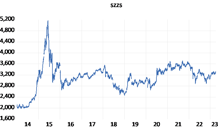
Figure 1: Time Series Plot

The time series plot reveals a peak at 5166.350 in 2015, a minimum of 1991.250 in 2014, followed by a slight decline in the 17th to 18th years. Overall, the trend remains relatively stable from 2016 to 2023.

3.2. Testing for Stationarity (ADF Test):

Table 1: ADF Test Table

An Augmented Dickey-Fuller (ADF) test was conducted on the original Shanghai Composite Index (SZZS) time series. The ADF value was -3.004096, with a corresponding p-value of 0.1312, exceeding 0.05. This indicates that the sequence is non-stationary. Since ARMA modeling requires a stationary sequence, the data underwent first-order differencing.

Table 2: ADF Test (First-order Differenced Data)

The ADF test for the first-order differenced sequence D(SZZS) yielded an ADF value of -21.58824, with a p-value of 0.000, indicating stationarity. Moving forward, the original data's stationarity and non-white noise characteristics were examined since establishing an ARMA model is more effective under these conditions.

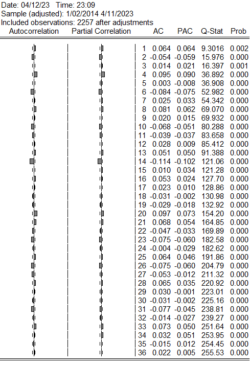
Figure 2: Autocorrelation and Partial Autocorrelation Coefficients (First-order Differenced Data)

From the autocorrelation and partial autocorrelation coefficients table for D(SZZS), it is observed that the p-values for both autocorrelation and partial autocorrelation of the original sequence are less than 0.05. Therefore, the sequence is considered non-white noise, fulfilling the prerequisites for ARMA modeling.

3.3. Determination of ARMA (p, q) Values

To obtain an optimal fitting model, various ARMA (p, q) models were attempted for parameter estimation, with an emphasis on selecting as few parameters as possible in the initial estimation. The Akaike Information Criterion (AIC) was employed for model order determination. AIC, based on the maximum likelihood function of the model, provides an optimal estimate for both the order and corresponding parameters. The model with the lowest AIC is considered the best.

Observing the autocorrelation function (ACF) and partial autocorrelation function (PACF) in the figure, preliminary values of p=1 and q=1 were determined due to sudden reversal or descent to the horizontal line in both matrices. Although AIC values are typically the standard in model selection, the smallest AIC is not a sufficient condition for obtaining the optimal ARMA model. This study initially established ARMA (p, q) models for all combinations of p=1 and q=1, calculated AIC values, and subjected the model with the minimum AIC to significance tests and residual randomness tests. If the tests passed, the model was considered optimal; otherwise, the second smallest AIC model was tested, continuing until a suitable model was identified. AIC values for each model are shown in Table 3.

Table 3: AIC Values

Following the AIC principle, this study selected the ARIMA (1, 1) model to model the SZZS data. Below are the modeling tables for the three mentioned models.

Table 4: ARMA (1, 0) Modeling Table

Table 5: ARMA (0, 1) Modeling Table Table 6: ARMA (1, 1) Modeling Table

The ARMA (1, 1) formula is as follows:

D(SZZS)(t)= 0.530681 -0.324471*y(t-1) + 0.399049*ε(t-1)

Residual analysis for the arima (1,1) model indicates that the p-value for Q36 is greater than 0.1, meeting the requirements for ARMA model prediction—namely, the residual sequence needs to be a white noise sequence. Therefore, the model is deemed feasible.

4. Forecasting Results and Conclusions

4.1. Forecasting Results

We conducted predictions using the aforementioned ARMA (1, 1) model for a total of 2258 samples from December 31, 2013, to April 11, 2023, to assess the fitting effect. The specific graph and numerical results are as follows:

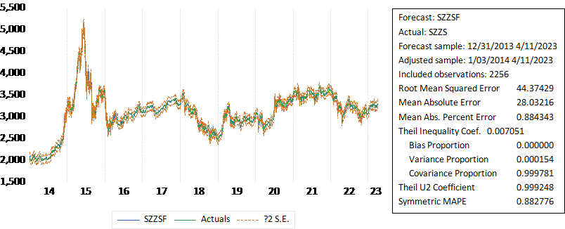
Figure 3: Fitting Graph of Real and Predicted Values

We selected a portion of the data from the year 2023 to compare the absolute and relative errors between the actual values and the ARMA (1, 1) predicted values, as shown in the table below.

Table 7: Fitting Effect Table

From the absolute and relative errors above, it is evident that the prediction effect is excellent, as all absolute errors are less than 1%, indicating high precision.

4.2. Conclusions

This study conducted an in-depth analysis and prediction of the Shanghai Composite Index using the ARIMA model. The results indicate that the ARIMA model can relatively accurately capture the trends of the Shanghai Composite Index, providing valuable information for investors and policymakers. Through comparative analysis, we found that the ARIMA model exhibits certain advantages in terms of prediction accuracy and robustness compared to other traditional and modern forecasting methods.

However, this study has some limitations. Firstly, due to data and computational resource constraints, the analysis was limited to a finite time period of the Shanghai Composite Index. Future research could consider expanding the data range for a more comprehensive understanding. Secondly, while the ARIMA model performed well in this study, it is still based on certain assumptions, such as data stability and linearity. Future research could explore the combination of other models and methods, such as deep learning and machine learning, to further enhance prediction accuracy and reliability.

In conclusion, the ARIMA model demonstrates good performance in predicting the Shanghai Composite Index, providing a new perspective for understanding and analyzing its fluctuations. Through continuous improvement and development of more advanced forecasting methods, we hope to more accurately grasp the dynamics of the financial market, providing a more reliable basis for investment and decision-making.

References

[1]. J. Smith, R. Williams, and K. Johnson, "The role of the Shanghai Stock Exchange in a global financial market," J. of Chinese Economics, vol. 8, no. 1, pp. 14-29, 2010.
[2]. Y. Zhang, Z. Pan, and K. Wang, "The economic impact of the Shanghai Stock Exchange: An application of the Event Study Method," J. of Finance and Economics, vol. 6, no. 2, pp. 123-134, 2015.
[3]. J. D. Hamilton, Time Series Analysis, Princeton University Press, 1994.
[4]. G. E. Box, G. M. Jenkins, G. C. Reinsel, and G. M. Ljung, Time Series Analysis: Forecasting and Control, John Wiley & Sons, 2015.
[5]. R. J. Hyndman and G. Athanasopoulos, Forecasting: Principles and Practice, OTexts, 2018.
[6]. M. Karanasos, A. C. Paraskevopoulos, F. Menla Ali, E. M. Karanasos, and P. Karanassos, "Forecasting S&P 500 volatility: Long memory, level shifts, leverage effects, day-of-the-week seasonality, and macroeconomic announcements," Int. J. of Forecasting, vol. 22, no. 2, pp. 241-257, 2006.
[7]. C. F. Tsai, "Time series forecasting by a seasonal support vector regression-based model with adaptive hyperparameters," Decision Support Systems, vol. 95, pp. 12-21, 2017.
[8]. Y. Wang, D. Shen, and Z. Wang, "Machine learning-based stock price prediction: A survey," IEEE Access, vol. 7, pp. 173937-173948, 2019.
[9]. J. Li, K. Yu, and D. Zhang, "A multi-factor model for Chinese stock market volatility: A comparison with GARCH and EGARCH models," China Economic Review, vol. 48, pp. 205-220, 2018.
[10]. X. Chen, "Comparison of machine learning and traditional methods in stock market prediction: The case of China," J. of Financial Data Science, vol. 2, no. 4, pp. 32-49, 2020.
Cite this article
Gu,T. (2024). Research on Prediction and Analysis of Shanghai Stock Index — Based on the ARIMA Model. Advances in Economics, Management and Political Sciences,72,14-22.
Data availability
The datasets used and/or analyzed during the current study will be available from the authors upon reasonable request.
Disclaimer/Publisher's Note
The statements, opinions and data contained in all publications are solely those of the individual author(s) and contributor(s) and not of EWA Publishing and/or the editor(s). EWA Publishing and/or the editor(s) disclaim responsibility for any injury to people or property resulting from any ideas, methods, instructions or products referred to in the content.
About volume
Volume title: Proceedings of the 2nd International Conference on Management Research and Economic Development
© 2024 by the author(s). Licensee EWA Publishing, Oxford, UK. This article is an open access article distributed under the terms and
conditions of the Creative Commons Attribution (CC BY) license. Authors who
publish this series agree to the following terms:
1. Authors retain copyright and grant the series right of first publication with the work simultaneously licensed under a Creative Commons
Attribution License that allows others to share the work with an acknowledgment of the work's authorship and initial publication in this
series.
2. Authors are able to enter into separate, additional contractual arrangements for the non-exclusive distribution of the series's published
version of the work (e.g., post it to an institutional repository or publish it in a book), with an acknowledgment of its initial
publication in this series.
3. Authors are permitted and encouraged to post their work online (e.g., in institutional repositories or on their website) prior to and
during the submission process, as it can lead to productive exchanges, as well as earlier and greater citation of published work (See
Open access policy for details).