1. Introduction

Stock prices serve as indicators of the present value of a stock for both buyers and sellers [1], hence potentially indicating fluctuations within the stock market. The efficient market hypothesis posits that market prices exhibit rapid responsiveness to publicly available information. However, this may not be the case in reality, due to the occurrence of unforeseeable circumstances. This study will primarily examine the empirical recession crises that occurred with the implementation of the Quantitative Easing (QE) program. The objective of this study is to examine the impact of quantitative easing initiatives on the stock market with regards to their potential implications for future investment.

This study is primarily motivated by the research conducted by Niederhoffer [2], who examined the impact of global events on stock market valuations. This study aims to conduct a scientific investigation using a Vector Autoregressive (VAR) model to ascertain the relationship between Quantitative Easing (QE) and stock prices. Additionally, it seeks to estimate the potential influence of QE on stock prices in the event of comparable crisis measures being implemented in the future. This study aims to examine the association between four quantitative easing programs and stock prices from 2007 to 2023, to prove the validity of relationship for a broader sample size. Moreover, the existing literature exhibits a research gap pertaining to the establishment of a connection between the beneficial impacts of a quantitative easing shock and the actual movements observed in stock prices. This study aims to quantitatively and comprehensively analyze the reaction by establishing a connection between the underlying policy motives and the prevailing economic conditions. This will be achieved by examining the impulse response functions within a structural VAR model.

2. Background

The stock market is fickle so that investors confront with uncertainties and try to catch all related information to predict the stock prices, aiming at decent returns [3]. Share price movement is not independent in nature. Specifically, the collective influence of book value, earnings per share, price-earnings ratio, and dividend yield accounts for 51.6% of the stock price of a corporation. The remaining unexplained portion requires more investigation. Aylward and Glen asserted that stock prices possess a wide-ranging predictive capability in terms of investment and the whole economy [4]. Hence, the efficacy of policies may be gauged by observing fluctuations in stock price indices. This research study aims to examine and evaluate the influence of past instances of Quantitative Easing (QE) programs on stock market valuations.

Quantitative Easing (QE) involves substantial acquisitions of assets, often include government debt with extended maturity periods, as well as private assets like corporate debt or asset-backed securities [5]. QE is commonly employed under atypical circumstances, such as when short-term nominal interest rates exhibit remarkable levels of low, zero, or even negative values, rendering them ineffectual to impact the market. In meanwhile, QE serves as an additional means of stimulating the economy through the reduction of long-term interest rates and the augmentation of liquidity in financial markets [6]. These factors are crucial in supporting the Federal Reserve's objectives of achieving full employment and maintaining price stability. The deployment of QE has a crucial role in stabilizing the economy during periods of downturn.

The Bank of Japan first introduced a Quantitative Easing (QE) policy to its zero interest rate policy between March 2001 and March 2006. Haltmaier, Martin, and Gust asserted that the implementation of QE has had a notable positive impact on macroeconomic circumstances in Japan, particularly while the official bank rate was either at or near zero [7]. This monetary policy measure has effectively contributed to the strengthening of the Japanese economy. Then, QE policy became a beneficial tool for some major central banks to mitigate recession crises by encouraging economic recovery, which in turn gradually unleashed credit and money creation [8]. In reaction to the two most recent recessions, the Federal Reserve implemented Quantitative Easing: the 2007-2009 recession and the 2020 recession precipitated by the coronavirus pandemic [6].

In the 2008 financial crisis, the US Federal Reserve significantly increased the size of its balance sheet by purchasing plenty of new assets and liabilities when the interest rate hit the zero lower bound [9]. Since November 2008, the Federal Reserve has begun purchasing assets as the first Quantitative Easing (QE1: December 2008 to March 2010), holding $600 billion in mortgage-backed assets [10]. The Federal Reserve held a large amount of bank debt, mortgage-backed securities, and Treasury notes, reaching a peak of $2.1 trillion in June 2010 [11]. To further stimulate the U.S. economy following the 2008 financial crisis and Great Recession, the Fed launched a second phase of Quantitative Easing (QE2: November 2010 to June 2011) in November 2010, buying $600 billion in long-maturity Treasury securities by the end of the second quarter of 2011 [12]. In September 2012, QE3 (September 2012 to October 2014) began operation, initially set at purchasing $40 billion per month for MBS and $45 billion per month for long-maturity Treasury securities [13]. In response to the COVID-19 epidemic, the Fed announced around $700 billion in QE4 (March 2020 to March 2022) via large-scale asset purchases on March 15, 2020 [14]. In QE4, the Fed has purchased nearly $6 trillion in assets [15].

3. Literature Review

Prior to the 2008 Financial Crisis, long-term interest rates drove the stock market [16], while since then QE seems to be the primary force behind the stock market recovery from a crisis. Bernanke and Reinhart demonstrated that QE can reduce the cost of borrowing by targeting a certain short-term interest rate [17]. QE helps to boost spending and eliminate recession through injection of new money into the economy [18]. The bank purchases financial assets from the private sector with newly issued central bank money. For every additional $1 billion in equity purchases from the private sector, the projected OLS model predicts that the stock price would rise by 0.021 dollars [19]. The effect is quite significant because the Federal Reserve was buying a large scale of assets each month. Stefanski used decision tree methodology and found that QE mostly affected the real economy by raising stock prices and lowering stock market volatility [20]. The primary benefits of QE are conceptual: an increase in Federal assets that is highly correlated with the S&P 500 Index; and a reduction in long-term interest rates, which similarly stimulates stock prices.

Tan and Kohli proposed a modified Constant Elasticity of Variance (CEV) class model and Auto-regression AR(1) model [21]. They found that the Federal Reserve's Quantitative Easing strategy has had a considerable detrimental influence on stock market volatility. They predicted a temporary spike in stock volatility at the end of QE2. The expected volatility ascent after the QE2 would make options more valuable. Chen and Yeh investigate industrial responses to both the 2008 global financial crisis and the COVID-19 epidemic [22]. Following QE announcements, the stock performance of the majority of industries began to improve from the negative effects of both occurrences, indicating that QE is successful in increasing investor confidence. Although stock prices continued to fall on March 20, 2020 as a result of the present economic crisis caused by the COVID 19 epidemic, the US S&P 500 index began to recover after March 23 as a result of Quantitative Easing, a powerful stimulus for the US Federal Reserve System (FED) [23]. Furthermore, using the Granger-Sims test, Hashemzadeh and Taylor discovered that the money supply and stock prices are characterized by a feedback system whereby fluctuations in the money supply cause variations in stock prices and vice versa [24]. Regarding to stock prices and interest rates, the causality seems to be unidirectional, mostly running from interest rates to stock prices.

According to Tawadros and Moosa, stock prices have a strong association with QE [25]. However, the estimated structural time series model revealed that missing variables other than QE influenced stock prices. One plausible rationale is that the implementation of QE might become consequential only after a particular threshold is surpassed. This could explain why the QE programs implemented by the Bank of England and the Bank of Japan, respectively, had no impact on FTSE100 and the NIKKEI 225. Via a Time-varying parametric framework, Al-Jassar and Moosa observed a general positive relationship between the Fed's balance sheet and stock prices, which was greatest during QE3 and lowest during QE2 [26]. The post-QE period (2015:10-2018:06) saw a weak correlation, which coincided with the Trump presidency, when the market is influenced by a variety of factors. According to Pham et al., certain of Trump's initiatives, such as deregulation and tax cuts, as well as increased government expenditure, benefit the stock market [27]. Furthermore, the performance of global stock markets, the performance of the US dollar, Fed funds rates, and changes in financial budgeting explain the majority of the variation in stock returns during the period of 2008 financial crisis with stable coefficients [28]. Bedikanli discovered that the FED's balance sheet and GDP effect stock prices statistically positively at the 1% level [29]. Thus, various factors in the economy environment significantly affect the stock market, which should be taken into account. In this instance, this inquiry will introduce a model to analyze the relationship between changes in stock prices and changes in FED’ s balance sheet, both over the last period.

4. Data

The dataset consists of the U.S. weekly data from 30 July 2007 to 24 July 2023. To analyze the effect of Quantitative Easing (QE) on stock prices, this research will estimate a vector auto-regression (VAR) model, with weekly time series data of QE and stock prices from 2007 to 2023. Based on past studies, the magnitude of QE was estimated by the size of Federal Reserve's balance sheet [30], denoted as Value. Stock prices were defined by the Standard and Poor's 500 stock index (S&P500) [31]. The natural logarithms of S&P500 was used, denoted as LSP500. All series became stationary after taking first difference.

5. Model

At the first stage, this study estimated a Vector auto-regression (VAR) model where endogenous variables included LSP500 and Value. The Co-integration Test found that there would be one co-integration equation between variables Value and LSP500, while the Johansen Procedure [32] test result indicated that there was no co-integration equation. Then, this investigation estimated a Vector Error Correction (ECM) model and failed to identify a significant error correction term. The model also had heteroscedasticity issue and non-normally distributed residuals.

To get a stationary data set and hence a valid VAR model, some diagnostic tests were taken on the natural log of stock prices (ln(S&P500)) and Federal Reserve's balance sheet (Value). The test results showed that both ln(S&P500) and Value were integrated order of 1 and became stationary after taking the first difference. Since HQ Hannan-Quinn (HQ) and Schwarz-Bayesian (BIC) criteria selected lags of 4 for the model, this research will use 4 lags throughout analysis. Then, the main model (1) is defined as below.

\( {y_{t}}=c+\sum _{j=1}^{p=4}{π_{j}}{y_{t-j}}+{ε_{t}} \)

\( (\begin{matrix}D1LSP50{0_{1t}} \\ D1Valu{e_{2t}} \\ \end{matrix})=(\begin{matrix}{c_{1t}} \\ {c_{2t}} \\ \end{matrix})+(\begin{matrix}π_{11}^{1} & π_{12}^{1} \\ π_{21}^{1} & π_{22}^{1} \\ \end{matrix})(\begin{matrix}D1LSP50{0_{1t-1}} \\ D1Valu{e_{2t-1}} \\ \end{matrix})+(\begin{matrix}π_{11}^{2} & π_{12}^{2} \\ π_{21}^{2} & π_{22}^{2} \\ \end{matrix})(\begin{matrix}D1LSP50{0_{1t-2}} \\ D1Valu{e_{2t-2}} \\ \end{matrix}) \) \( +(\begin{matrix}π_{11}^{3} & π_{12}^{3} \\ π_{21}^{3} & π_{22}^{3} \\ \end{matrix})(\begin{matrix}D1LSP50{0_{1t-3}} \\ D1Valu{e_{2t-3}} \\ \end{matrix})+(\begin{matrix}π_{11}^{4} & π_{12}^{4} \\ π_{21}^{4} & π_{22}^{4} \\ \end{matrix})(\begin{matrix}D1LSP50{0_{1t-4}} \\ D1Valu{e_{2t-4}} \\ \end{matrix})+(\begin{matrix}{ε_{1t}} \\ {ε_{2t}} \\ \end{matrix}) \) (1)

where the D1LSP500 refers to the first difference in ln(S&P500) and D1Value refers to the first difference in Value. is the stochastic component.

6. Data Analysis

Both stock prices (LSP500) and Fed’s balance sheet (Value) show clearly a strong positive trend and positive correlation over time. The Value appears to suffer structural break problems at the second half of data set.

After taking the first difference, stock prices (D1LSP500) and Fed’s balance sheet (D1Value) fluctuate around zero (Appendix 1) and S&P500 index is far less volatile than FED balance sheet. Clearly, there are time lags between variables fluctuations. There is a slight positive relationship between endogenous variables over time in model (1). The Appendix 2 is indicative of several outliers problems in the data set.

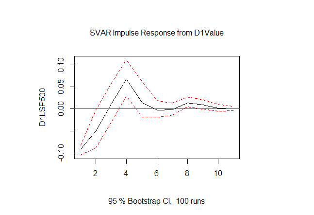
Figure 1: SVAR Impulse response functions of D1LSP500 to D1Value for model (1)

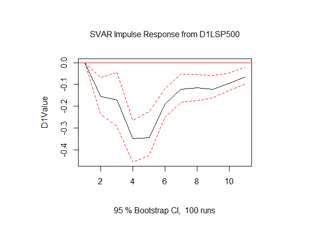
Figure 2: SVAR Impulse response functions of D1Value to D1LSP500 for model (1)

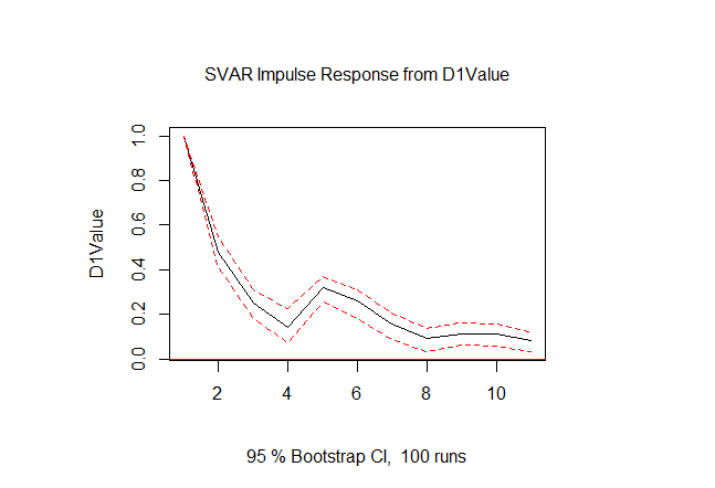
Figure 3: SVAR Impulse response functions of D1Value to D1Value for model (1)

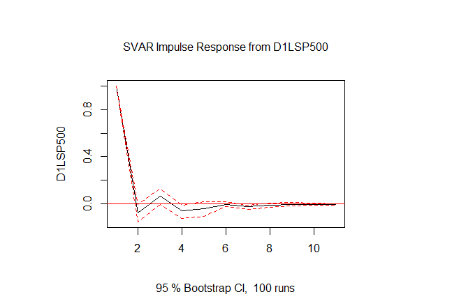
Figure 4: SVAR Impulse response functions of D1LSP500 to D1LSP500 for model (1)

In order to estimate the structural VAR for further interpretation of shocks [33], short-run restrictions between contemporaneous variables on the model were employed. The FED ’s balance sheet shocks cannot contemporaneously impact stock prices and changes in stock prices shocks cannot immediately affect FED ’s balance sheet.

From the figure 1, a standard deviation shock to D1Value results in a dramatic fluctuation in the D1LSP500 and then converges back to zero at the fifth period. With a shock of changes in the FED balance sheet by 1 billion, the S&P500 index descends by almost 1% in 1 week, and will fluctuate and return to original index in six weeks. In the figure 2, the initial shock of 1% change in the S&P500 index leads to a significant drop in the FED balance sheet in the first five periods, approximately 248.76 millions and then the impact takes 15 periods return to zero. A significant rise in the D1Value following a shock in D1Value and the impact converges back almost to zero in 3 months, as shown in figure 3. By contrast, figure 4 points out that a shock in the D1LSP500 causes a drastic increase in D1LSP500 and then the impact dies quickly at the second period.

In addition, the Granger Causality test was employed on model (1), that some econometricians defined it as predictive causality [34], to determine whether a time series can predict another series [35]. The test results demonstrate that series D1Value and D1LSP500 interchangeably Granger cause each other. However, the variance decomposition analysis indicates that the forecast error variance of D1LSP500 can not be explained by exogenous shocks to D1Value, while shocks to D1LSP500 can explain small parts of forecast error variance of D1Value. This results are compatible with the impulse response analysis that D1LSP500 has little response to shocks in D1Value, compared with the inverse direction.

The Fan charts give the forecasting distribution of a variable based on the all available information [36]. The Fan chart respectively predicts that the variable D1Value will go up and D1LSP500 will remain stable at faint positively above zero.

7. Diagnostic Tests

The VAR model (1) has no serial correlation problem at 1% significance level. Meanwhile, the ARCH test shows the existence of heteroscedasticity issue. Normality test shows that residuals of the Model (1) is not normally distributed. The stability measures show that series D1LSP500 and D1Value are stable without structural break despite of a large negative fluctuation in the D1LSP500 in the 2008 Financial crisis. These issues do not impress the credibility of the model (1).

Furthermore, data set was fragmented into 4 periods corresponding to 4 QE implementation separately to check the robustness of prediction results. During the QE1, all results were robust and consistent with the average results. However, the forecast error variance of D1LSP500 became significantly explainable by shocks to D1Value. The 2008 Financial crisis was perceived as the most severe global recession since the Great Depression [37]. In the late 2008, lack of investor confidence and dwindling credit availability prompted a sharp fall in stock and commodity prices [38], causing numerous banks and businesses bankrupt. Accordingly, the contemporaneous variance decomposition dissection may potentially verify the authority of QE1 on the recovery of the financial market, via the S&P500 index.

In the QE2 period, the impulse response for D1Value to a shock of 1% rise in D1LSP500 became inverse. The variance decomposition analysis indicates that the forecast error variance of D1Value cannot be explained by exogenous shocks to D1LSP500 during the QE2. The United States' recovery was still sporadic when QE2 was introduced. Even though the stock market had rebounded from its 2008 lows, unemployment remained high [39]. The improved financial market environment after the QE1 and reduced balance sheet in the QE2 [12] may explain the short-term boost in S&P500 index when QE2 was implemented.

In the period QE3, a D1LSP500 shock will no not cause a persistent fall in the D1Value but a moderate fluctuation. Also, D1Value became fluctuated following a shock in D1Value, but still amount almost above zero. The QE3 period experienced a similar variance decomposition analysis as during the QE2. In 2012, the economy was still fallow. For instance, the growth rate of labor market improvement was quite low and the inflation rate fell short of the target level. Hence, the QE3 program was designed on the concept of state-contingent, which would continue until significant improvements in the labor market outlook [40]. The state-contingent concept for QE3 could explain why stock market could impact Fed’s balance sheet and its volatility. Both QE2 and QE3 were designed to aid revive the economy following the 2008 Financial crisis, such that these periods saw the similar variance decomposition analysis that S&P500 and Fed’s balance sheet do not influence each other significantly.

In the QE4, overall patterns from the impulse response functions are robust and coherent with the average results but the effects of shocks are relatively more significant than had ever before. The Federal Reserve mentioned in its statement that the coronavirus outbreak has severely damaged communities and disrupted economic activity worldwide [41]. The large-scale asset purchases reached 6 trillions during the QE4 [15], which is the largest volume over the past QE programs. This fact potentially explains the relatively more significant impact between variables, compared to past periods.

8. Discussion

Overall, this study found a positive significant correlation between QE programs and S&P500 index, which is consistent with Phillips [19] and Stefanski [20], even though there were lags between shocks and responses. As mentioned above, Stefanski found that QE mainly raised Federal assets strongly correlated with the S&P 500 Index. The injection of large amount of money into the economy lowered the long-term interest rates and thus raised the stock prices. The adjustment time for long-term interest rates may potentially illuminate the lagged impulse response of stock prices to a shock in QE. Additionally, Alam and Uddin proved a significant negative relationship between interest rates and share price across developed and developing countries [42]. Further research could expand the subject to include both short- and long-term interest rates to prove the causes of lagged responses to shocks.

Brooks, Patel, and Su discovered that when unfavorable news about unpredictable events is publicly announced, equity prices reverse following the initial negative price reaction, suggesting that investors overreacted [43]. Their discovery perfectly match the research findings, as shown in Figure 1, even though the impulse responses almost return to zero at the fifth period. Particularly during QE1, the stock market responded to a shock in the Fed's balance sheet over a comparatively longer period of time than following programs.

Moreover, Tan and Kohli predictions on QE2 were actualized in the financial market, and even validated in further crises with implementation of QE [21]. The impulse response function (Figure 1) has shown that a positive shock in QE will make assets more valuable after a quick fall in stock prices, possibly owing to an ascent in the stock volatility at the end of QE program.

Bedikanli analysed the effect of Federal Reserve Banks (FED)’ s large-scale asset purchase (LSAP) on stock prices (S&P500) in the US [29]. By using the Error Corrected (EC) version of the Autoregressive distributed-lagged model (ADL), the results show that there is a statistically significant positive long-run relationship between the FED’ s balance sheet and stock prices. However, this inquiry found ambiguous evidence of the existence of co-integration equation and no significant error correction term between the same endogenous variables. This difference could be explained by the distinguished samples since Bedikanli analyzed quarterly data from 2009Q1 to 2018Q4.

Furthermore, this study found bi-directional Granger-cause effect on both stock prices and Fed’s balance sheet, which is consistent with Hashemzadeh and Taylor, who discovered a bi-directional feedback system between money supply and stock prices [24]. Although money supply is not equal to Fed’ s balance sheet, QE programs inject money into the economy by raising assets. There could be a linear relationship between them and this could be deeply analyzed in the future research.

According to Tawadros and Moosa, QE may only have an impact once a specific threshold has been reached [25]. This interpretation could potentially clarify hitherto findings in this investigation. In model (1) with data between 2007 and 2023, QE had significant effects on S&P500 index at 5% level. Nevertheless, when dividing the data set into four distinct periods to align with the four quantitative easing (QE) programs, this study observed that the Federal Reserve's balance sheet had a negligible effect on the S&P 500 index during the QE2 and QE3 periods. The purpose of the QE2 and QE3 programs, which aimed to further stimulate the economy following the 2008 financial crisis, might account for these behaviors. QE2 shrunk the balance sheet compared with QE1 [12], and QE3 was implemented with the intention of strengthening the labor market by employing the state-contingent approach [40]. Meanwhile, in QE4 period, S&P500 responded only significantly to changes in 4th lagged Fed’s balance sheet at 5% level. The delayed response in S&P500 might result from the lockdown and recession during the Covid-19 pandemic [41] when people lost confidence about market.

9. Conclusion

To sum up, this research aimed to analyze the effect of historical Quantitative Easing (QE) programs on U.S. stock price index S&P500. Based on quantitative analysis on a structural VAR model, S&P500 index responded significantly to shocks in QE during the QE1 and QE4 periods. S&P500 would drop quickly in two months and then rise significantly over long time. Beyond previous research, this article established a link between data analysis and the motivations of historical quantitative easing programs. Hopefully, the findings will enable investors to make judicious investments that yield respectable returns, even in times of recession. This research clearly illustrates the lagged effect of QE programs on S&P500 index, while it also raises the potential omitted variables bias issue. There are several economic factors that have a substantial impact on the stock market. For instance, a positive significant coefficient was ascertained on the constant term in model (1), defined as linear trend, which might be potentially explained by climbing inflation over time. To better comprehend the inferences of these results, future studies should consider broader economic indicators and contemporaneous policies that affect the market. Finally, further research should concentrate on dissecting the relationship between short-term and long-term interest rates and lagged responses in the financial market.

References

[1]. Pinsent, W. (2020). Understanding Stock Prices and Values. [online] Investopedia. Available at: https://www.investopedia.com/articles/stocks/08/stock-prices-fool.asp.
[2]. Niederhoffer, V. (1971). The Analysis of World Events and Stock Prices. The Journal of Business, [online] 44(2), pp.193–219. Available at: https://www.jstor.org/stable/2351663?saml_data=eyJzYW1sVG9rZW4iOiJlMDM3MGM0MC0zNTczLTRhNTktYmM0OS1kMTkzNjExNmVmZGYiLCJpbnN0aXR1dGlvbklkcyI6WyIzZGVlYmI1NC0yMDMwLTQ3YjgtYjhjNi0wN2E3NzQ3NDFlZGEiXX0 [Accessed 26 Oct. 2023].
[3]. Malhotra, N. and Tandon, K. (2013). Determinants of Stock Prices: Empirical Evidence from NSE 100 Companies. IRACST- International Journal of Research in Management & Technology (IJRMT), 3(2249-9563).
[4]. Aylward, A. and Glen, J. (2000). Some International Evidence on Stock Prices as Leading Indicators of Economic Activity. Applied Financial Economics, 10(1), pp.1–14. doi:https://doi.org/10.1080/096031000331879.
[5]. Williamson, S. (2017). Quantitative Easing: How Well Does This Tool Work? [online] Stlouisfed.org. Available at: https://www.stlouisfed.org/publications/regional-economist/third-quarter-2017/quantitative-easing-how-well-does-this-tool-work.
[6]. Congressional Budget Office (2021). How the Federal Reserve’s Quantitative Easing Affects the Federal Budget | Congressional Budget Office. [online] www.cbo.gov. Available at: https://www.cbo.gov/publication/58457 [Accessed 25 Sep. 2023].
[7]. Haltmaier, J., Martin, R. and Gust, C. (2008). Authorized for public release by the FOMC Secretariat 7. Effects of the Bank of Japan’s Quantitative Easing Policy on Economic Activity. [online] Available at: https://www.federalreserve.gov/monetarypolicy/files/FOMC20081212memo07.pdf#:~:text=From%20March%20of%202001%20through%20March%20of%202006%2C [Accessed 24 Oct. 2023].
[8]. Sławiński, A. (2016). The role of the ECB’s QE in alleviating the Eurozone debt crisis. Wydawnictwo Uniwersytetu Ekonomicznego we Wrocławiu, [online] (428), pp.236–250. Available at: https://www.ceeol.com/search/article-detail?id=426214 [Accessed 24 Oct. 2023].
[9]. Alloway, T. (2008). The Unthinkable Has Happened. [online] www.ft.com. Available at: https://www.ft.com/content/d0908415-61b8-3cd7-9ba6-09df9dc9042e [Accessed 24 Oct. 2023].
[10]. BOARD OF GOVERNORS of the FEDERAL RESERVE SYSTEM (2008). Federal Reserve Announces It Will Initiate a Program to Purchase the Direct Obligations of housing-related government-sponsored Enterprises and mortgage-backed Securities Backed by Fannie Mae, Freddie Mac, and Ginnie Mae. [online] Board of Governors of the Federal Reserve System. Available at: https://www.federalreserve.gov/newsevents/pressreleases/monetary20081125b.htm [Accessed 24 Oct. 2023].
[11]. Ali, A.O.R.I.C.H.A. (2015). Quantitative Monetary Easing - the History and Impacts on Financial Markets. www.academia.edu. [online] Available at: https://www.academia.edu/6943181 [Accessed 24 Oct. 2023].
[12]. Censky, A. (2010). Quantitative Easing 2 Is here: Federal Reserve - Nov. 3, 2010. [online] money.cnn.com. Available at: https://money.cnn.com/2010/11/03/news/economy/fed_decision/index.htm [Accessed 20 Oct. 2023].
[13]. Zumbrun, J. (2012). Fed Undertakes QE3 with $40 Billion Monthly MBS Purchases. Bloomberg.com. [online] 13 Sep. Available at: https://www.bloomberg.com/news/articles/2012-09-13/fed-plans-to-buy-40-billion-in-mortgage-securities-each-month?leadSource=uverify%20wall [Accessed 24 Oct. 2023].
[14]. Liesman, S. (2020). Federal Reserve cuts rates to zero and launches massive $700 billion Quantitative Easing program. [online] CNBC. Available at: https://www.cnbc.com/2020/03/15/federal-reserve-cuts-rates-to-zero-and-launches-massive-700-billion-quantitative-easing-program.html [Accessed 21 Oct. 2023].
[15]. JD Henning (2022). The FED Ends The $6 Trillion QE4: How The Markets May React | Seeking Alpha. [online] seekingalpha.com. Available at: https://seekingalpha.com/article/4494773-fed-ends-6-trillion-qe4-how-markets-react [Accessed 21 Sep. 2023].
[16]. Bhar, R., Malliaris, A. (Tassos) G. and Malliaris, M. (2016). Quantitative Easing and the U.S. Stock Market: A Decision Tree Analysis. [online] Social Science Research Network. Available at: https://papers.ssrn.com/sol3/papers.cfm?abstract_id=2760029 [Accessed 24 Sep. 2023].
[17]. Bernanke, B.S. and Reinhart, V.R. (2004). Conducting Monetary Policy at Very Low Short-Term Interest Rates. American Economic Review, 94(2), pp.85–90. doi:https://doi.org/10.1257/0002828041302118.
[18]. Benford, J., Berry, S., Nikolov, K., Young, C., & Robson, M. (2009). Quantitative easing. Bank of England. Quarterly Bulletin, 49(2), 90.
[19]. Phillips, G. (2022). The Effect of Quantitative Easing on the US Stock Market and Wealth Inequality.
[20]. Stefański, M. (2022). Macroeconomic effects and transmission channels of quantitative easing. Economic Modelling, 114, p.105943. doi:https://doi.org/10.1016/j.econmod.2022.105943.
[21]. Tan, J. and Kohli, V. (2011). The Effect of Fed’s Quantitative Easing on Stock Volatility. SSRN Electronic Journal. doi:https://doi.org/10.2139/ssrn.2215423.
[22]. Chen, H.-C. and Yeh, C.-W. (2021). Global financial crisis and COVID-19: Industrial reactions. Finance Research Letters, 42, p.101940. doi:https://doi.org/10.1016/j.frl.2021.101940.
[23]. Hong, S. (2021). Analysis of the Ripple Effect of the US Federal Reserve System’s Quantitative Easing Policy on Stock Price Fluctuations. https://web.s.ebscohost.com/abstract?direct=true&profile=ehost&scope=site&authtype=crawler&jrnl=27136434&AN=150048716&h=Tuu2MAI2X0kHhWZ764%2b8Od2ZuM4nyrOomuwPozT%2b88Xj5pRfg4UhbMPW8jtaxaMQ8BaKgU4IES31VBcc9mXs%2fw%3d%3d&crl=c&resultNs=AdminWebAuth&resultLocal=ErrCrlNotAuth&crlhashurl=login.aspx%3fdirect%3dtrue%26profile%3dehost%26scope%3dsite%26authtype%3dcrawler%26jrnl%3d27136434%26AN%3d150048716.
[24]. Hashemzadeh, N. and Taylor, P. (1988). Stock prices, Money supply, and Interest rates: the Question of Causality. Applied Economics, 20(12), pp.1603–1611. doi:https://doi.org/10.1080/00036848800000091.
[25]. Tawadros, G.B. and Moosa, I.A. (2022). A Structural Time Series Analysis of the Effect of Quantitative Easing on Stock Prices. International Journal of Financial Studies, 10(4), p.114. doi:https://doi.org/10.3390/ijfs10040114.
[26]. Al-Jassar, S.A. and Moosa, I.A. (2018). The effect of quantitative easing on stock prices: a structural time series approach. Applied Economics, 51(17), pp.1817–1827. doi:https://doi.org/10.1080/00036846.2018.1529396.
[27]. Pham, H.N.A., Ramiah, V., Moosa, N., Huynh, T. and Pham, N. (2018). The financial effects of Trumpism. Economic Modelling, [online] 74, pp.264–274. doi:https://doi.org/10.1016/j.econmod.2018.05.020.
[28]. Villanueva, M. (2015). Quantitative Easing and US Stock Prices. SSRN Electronic Journal. doi:https://doi.org/10.2139/ssrn.2656329.
[29]. Bedikanli, M. (2020). Quantitative easing and US stock prices : A study on unconventional monetary policy and its long-term effects on stocks (Dissertation). Retrieved from https://urn.kb.se/resolve?urn=urn:nbn:se:umu:diva-167940.
[30]. Statista (2023). U.S. Federal Reserve Balance Sheet 2007-20203. [online] Statista. Available at: https://www.statista.com/statistics/1121448/fed-balance-sheet-timeline/.
[31]. Yahoo! Finance (2023). S&P 500 (^GSPC) Historical Data - Yahoo Finance. [online] finance.yahoo.com. Available at: https://finance.yahoo.com/quote/%5EGSPC/history?period1=1664786563&period2=1696322563&interval=1mo&filter=history&frequency=1mo&includeAdjustedClose=true [Accessed 25 Oct. 2023].
[32]. Johansen, S. (1991). Estimation and Hypothesis Testing of Cointegration Vectors in Gaussian Vector Autoregressive Models. Econometrica, 59(6), p.1551. doi:https://doi.org/10.2307/2938278.
[33]. Lütkepohl, H. (2010). Impulse response function. Macroeconometrics and Time Series Analysis, pp.145–150. doi:https://doi.org/10.1057/9780230280830_16.
[34]. Diebold, F.X. (2007). Elements of Forecasting. South-Western Pub.
[35]. Granger, C. W. J. (1969). "Investigating Causal Relations by Econometric Models and Cross-spectral Methods". Econometrica. 37 (3): 424–438. doi:10.2307/1912791. JSTOR 1912791.
[36]. Julio, J. M. (2006). The Fan Chart: Implementation, Usage and Interpretation. Revista Colombiana de Estadistica, 29(1), 109.
[37]. Temin, P. (2010). The Great Recession & the Great Depression. MIT Open Access Articles. [online] Available at: https://dspace.mit.edu/bitstream/handle/1721.1/60250/Temin-2010-The%20Great%20Recession.pdf [Accessed 27 Oct. 2023].
[38]. Evans-Pritchard, A. (2007). Dollar Tumbles as Huge Credit Crunch Looms. [online] www.telegraph.co.uk. Available at: https://www.telegraph.co.uk/expat/4204516/Dollar-tumbles-as-huge-credit-crunch-looms.html.
[39]. U.S. Bureau of Labor Statistics (2018). Bureau of Labor Statistics Data. [online] Bls.gov. Available at: https://data.bls.gov/timeseries/lns14000000.
[40]. Federal Reserve Bank of St. Louis (2018). QE3: Data-Driven, Not Date-Driven | Annual Report 2017 | St. Louis Fed. [online] www.stlouisfed.org. Available at: https://www.stlouisfed.org/annual-report/2017/qe3-data-driven-not-date-driven [Accessed 28 Oct. 2023].
[41]. Federal Reserve (2020). Federal Reserve Issues FOMC Statement. [online] Board of Governors of the Federal Reserve System. Available at: https://www.federalreserve.gov/newsevents/pressreleases/monetary20200315a.htm.
[42]. Alam, M.M. and Uddin, G. (2009). Relationship between Interest Rate and Stock Price: Empirical Evidence from Developed and Developing Countries. [online] papers.ssrn.com. Available at: https://papers.ssrn.com/sol3/papers.cfm?abstract_id=2941281.
[43]. Brooks, Raymond M., Patel, A. and Su, T. (2003). How the Equity Market Responds to Unanticipated Events*. The Journal of Business, 76(1), pp.109–133. doi:https://doi.org/10.1086/344115.
Cite this article
Tang,L. (2024). The Impact of Quantitative Easing on Stock Prices in the U.S. Stock Market - Structural VAR Model Analysis. Advances in Economics, Management and Political Sciences,72,117-127.
Data availability
The datasets used and/or analyzed during the current study will be available from the authors upon reasonable request.
Disclaimer/Publisher's Note
The statements, opinions and data contained in all publications are solely those of the individual author(s) and contributor(s) and not of EWA Publishing and/or the editor(s). EWA Publishing and/or the editor(s) disclaim responsibility for any injury to people or property resulting from any ideas, methods, instructions or products referred to in the content.
About volume
Volume title: Proceedings of the 2nd International Conference on Management Research and Economic Development
© 2024 by the author(s). Licensee EWA Publishing, Oxford, UK. This article is an open access article distributed under the terms and
conditions of the Creative Commons Attribution (CC BY) license. Authors who
publish this series agree to the following terms:
1. Authors retain copyright and grant the series right of first publication with the work simultaneously licensed under a Creative Commons
Attribution License that allows others to share the work with an acknowledgment of the work's authorship and initial publication in this
series.
2. Authors are able to enter into separate, additional contractual arrangements for the non-exclusive distribution of the series's published
version of the work (e.g., post it to an institutional repository or publish it in a book), with an acknowledgment of its initial
publication in this series.
3. Authors are permitted and encouraged to post their work online (e.g., in institutional repositories or on their website) prior to and
during the submission process, as it can lead to productive exchanges, as well as earlier and greater citation of published work (See
Open access policy for details).