1. Introduction

In recent years, the outbreak of the COVID-19 epidemic has seriously affected the operations and production of various industries around the world, and has also had a greater impact on GDP. In order to alleviate the legacy impact of this turbulent period on various enterprises and prevent enterprises from falling into financial crisis, risk portfolio management of enterprises has become an urgent problem to be solved [1]. Effective risk management assessment of the portfolio is the key to the success of the project portfolio, which is consistent with the strategic objectives of the investor [2]. As a type of investment portfolio planning, the index model well solves the problem of high cost caused by complex calculation, and it involves tracking specific market indexes and taking into account the market environment risks outside the company [3]. It can better conduct a reasonable evaluation of multiple assets, thereby helping to reduce the risk of the asset portfolio.

As a risk portfolio management method, the index model divides risk uncertainty into system macro and company internal micro factors. At the same time, it uses the return rate of stock indexes such as the S&P 500 as an effective proxy indicator of common macroeconomic factors. Enables businesses to track a specific market index to achieve returns similar to that index [4]. This model is estimated through regression analysis of excess returns. The constructed risk portfolio is composed of an active investment portfolio and a consumer market portfolio. In this way, the market index portfolio can be used to improve the diversification level of the entire portfolio and increase the diversification level of the entire portfolio. Portfolios involve multiple assets to avoid investors being overly concentrated in one area, thereby reducing risk.

Among them, consumption, as an important part of GDP, has also been affected by the epidemic and has experienced relatively strong fluctuations [5]. The consumption industry is selected as the research object, mainly considering that consumption is related to people's needs [6]. The consumption industry is divided into daily consumption and optional consumption. For daily consumption, even during the economic downturn caused by the epidemic, the daily consumption industry has relatively stable demand than other industries. For example, some consumer companies produce daily necessities, and there is still demand even in the economic downturn. It has certain anti-cyclicality. For optional consumption, the optional consumption industry can reflect social trends and economic conditions to a certain extent. The overall economic conditions of society determine the purchasing power of such products. Therefore, studying this industry can reveal some more valuable macro information. In addition, there are many large consumer companies with global markets and operations around the world, which can reduce the impact of regional economics on risk planning.

2. Methodology

2.1. Analysis of the Investment Mechanism of Index Model Theory

In the past, investors usually used the company's financial data and indicators to evaluate investment risks, ignoring the impact of the external market on the investment portfolio to a certain extent. The index model is not only concerned with the weight allocation of the active portfolio of the portfolio, but also focuses on the market index used to measure the market performance, comprehensively assessing the risk level of the stock and reducing the specific risk [7]. The most important thing about index models is timing, which provides a framework for macro and security analysis, which is essential for the efficiency of an optimal portfolio.

The index model framework separates the sources of fluctuations in macro forecasts and return expectations for securities, reducing analytical variability [8]. Based on the above investment philosophy, the index model is applied to the portfolio model, and the risk is measured by input data:

(1) Macroeconomic analysis, which is mainly used to estimate specific market indices and premiums.

(2) Statistical analysis for estimating β coefficients and residual variance values.

(3) Prediction of security-specific returns based on security characteristic lines, used to estimate α value, reflecting the incremental risk premium from the information found in the analysis [9].

The above steps are the preparatory steps of the exponential model framework, which provide a theoretical basis for subsequent research.

2.2. Modeling

2.2.1. Exponential Model

The index model, which provides a decentralized perspective for investors to conduct investment activities, was first proposed by Sharp. The main point of this model is that it is representative of the market, by tracking the market index, so as to make a reasonable analysis of the market, and reduce the risk of a specific stock or industry.

The capital asset pricing model and linear regression are used to estimate the sensitivity of specific securities to market indexes, and the excess return of securities in the consumer industry is regressed to obtain the regression equation:

\( {R_{i}}(t)={α_{i}}+{β_{i}}{R_{M}}(t)+{e_{i}}(t) \) (1)

Where \( {R_{i}}(t) \) is the excess return of securities in the consumer sector, and the intercept α indicates the expected excess return of the consumer sector when the excess return of the market index is 0. β represents the sensitivity factor, which represents the systemic risk of an asset relative to the market and measures the sensitivity of an asset relative to the market portfolio. Considering that all the assets in the market form a market portfolio, M is used to represent the market index, and the excess return is \( {R_{M}} \) , which represents the average return of the entire market. \( {e_{i}} \) is referred to as residual values and represents other risks that have been stripped by the system and are not accounted for by the model.

2.2.2. The Optimal Risk Mix under the Index Model

Under the index model, the optimal risk portfolio is determined by the capital market line, and the goal is to maximize the Sharpe ratio through the selection of portfolio weights to obtain the portfolio Sharpe ratio:

\( E({R_{p}})={α_{p}}+E({R_{p}}){β_{p}}=\sum _{i=1}^{n+1}{ω_{i}}{α_{i}}+E({R_{M}})\sum _{i=1}^{n+1}{ω_{i}}{β_{i}} \) (2)

\( {σ_{p}}={[{{β_{p}}^{2}}{{σ_{M}}^{2}}+{σ^{2}}({e_{p}})]^{\frac{1}{2}}}={[{{{σ_{M}}^{2}}(\sum _{i=1}^{n+1}{w_{i}}{β_{i}})^{2}}+\sum _{i=1}^{n+1}{{ω_{i}}^{2}}{σ^{2}}({e_{i}})]^{\frac{1}{2}}} \) (3)

\( {S_{p}}=\frac{E({R_{p}})}{{σ_{p}}} \) (4)

Maximizing the Sharpe ratio on the capital market line means \( {σ_{p}} \) , the smallest point is the optimal risk portfolio, where \( {σ_{p}} \) represents the variance of the risk portfolio.

2.2.3. Portfolio Optimization Process

Calculate the original position for each security of the active portfolio:

\( ω_{i}^{0}=\frac{{α_{i}}}{{σ^{2}}({e_{i}})} \) (5)

Adjust the original weights so that the combined weights are 1:

\( {ω_{i}}=\frac{ω_{i}^{0}}{\sum _{i=1}^{n}ω_{i}^{0}} \) (6)

Calculate the α value of the positive combination:

\( {α_{A}}=\sum _{i=1}^{n}{ω_{i}}{α_{i}} \) (7)

Calculate positive combination residuals:

\( {σ^{2}}({e_{A}})=\sum _{i=1}^{n}{{ω_{i}}^{2}}{σ^{2}}({e_{i}}) \) (8)

Calculate the original position of the active combination:

\( ω_{A}^{0}=\frac{\frac{{α_{A}}}{{σ^{2}}({e_{A}})}}{\frac{E({R_{M}})}{{{σ_{M}}^{2}}}} \) (9)

Calculate the β value of positive combinations:

\( {β_{A}}=\sum _{i=1}^{n}{ω_{i}}{β_{i}} \) (10)

Adjust the original position of the active combination:

\( ω_{A}^{*}=\frac{ω_{A}^{0}}{1+(1-{β_{0}})ω_{A}^{0}} \) (11)

The weight of the optimal risk portfolio at this point:

\( ω_{M}^{*}=1-ω_{A}^{*} \) ; \( ω_{i}^{*}=ω_{A}^{*}{ω_{i}} \) (12)

2.3. Metric Selection and Data Sources

When researching the portfolio of the consumer sector, the author chooses Costco, Walmart as the two representative stocks of daily consumption, and Lululemon and Under Armour as the representative stocks of optional consumption. Among them, Costco is the largest chain of membership-based warehouse stores in the United States, and Wal-Mart is one of the world's largest retailer giants, both of which have a leading position in the daily consumption industry and have business all over the world, and both companies have relatively strong brand reputation, and are two strong representative companies in the daily consumption industry. For optional consumption, Under Armour and Lululemon are both well-known sports brands and have great influence. Under Armour offers a wide range of sports and leisure products with a wide range of market lines and a strong brand presence in the sports and exercise space thanks to partnerships with some of the most well-known athletes. Lululemon specializes in the design and sale of high-quality, high-end sports equipment and yoga apparel, and is an important brand in the consumer discretionary industry. The four companies selected have strong influence in the corresponding industry and have good representativeness.

The data is selected from October 2018 to November 2023, and the opening and closing prices are counted on a monthly basis, and the average monthly yield is calculated. All data comes from the iFinD database, which uses the S&P 500 as the market characteristic index to represent market conditions, and uses short-term U.S. Treasuries to represent risk-free assets.

3. Results and Discussion

3.1. Empirical Analysis

Walmart (WMT):

\( {R_{WMT}}={α_{WMT}}+{β_{WMT}}{R_{sp500}}(t)+{e_{WMT}}(t) \) (13)

The above equation describes the linear relationship between Walmart's excess return and changes in economic conditions represented by the S&P 500 return.

Table 1: Regression statistics of Walmart.

As can be seen from Table 1, the correlation between Walmart and the S&P 500 Index reaches 0.5588, indicating that Walmart does not move significantly in the same direction with the fluctuations of the S&P 500 Index \( {R^{2}} \) . is 0.3122, indicating that the variance of the S&P 500 index can explain approximately 31.22% of Walmart's. The adjusted is \( {R^{2}} \) slightly smaller than the original \( {R^{2}} \) , corrected for using α and β estimates rather than true values. The regression result is shown in Figure 1.

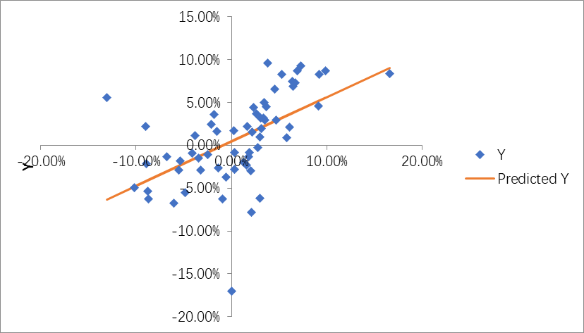
Figure 1: The correlation between Walmart and the S&P 500 Index.

COSTCO:

\( {R_{COSTCO}}={α_{COSTCO}}+{β_{COSTCO}}{R_{sp500}}(t)+{e_{COSTCO}}(t) \) (14)

Table 2: Regression statistics of Costco.

The correlation between Costco and the S&P 500 Index (see Table 2) reaches 0.6784, indicating that Costco moves in the same direction as the S&P 500 Index fluctuates. \( {R^{2}} \) is 0.4602, indicating that the variance of the S&P 500 index can explain approximately 46.02% of Costco. The regression result is shown in Figure 2.

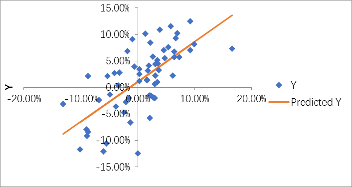
Figure 2: The correlation between Costco and the S&P 500 Index.

Under Armor (UA)

\( {R_{UA}}={α_{UA}}+{β_{UA}}{R_{sp500}}(t)+{e_{UA}}(t) \) (15)

Table 3: Regression statistics of Under Armor.

In the same way, it can be seen from Table 3 that the correlation between Under Armor and the S&P 500 Index reaches 0.626 2, indicating that Under Armor moves in the same direction as the S&P 500 Index fluctuates. \( {R^{2}} \) is 0.3921, indicating that the variance of the S&P 500 index can explain about 39.21% of Under Armor. The regression result is shown in Figure 3.

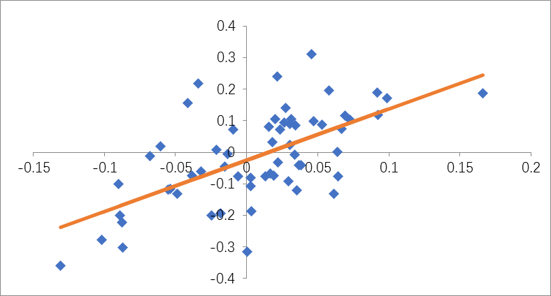
Figure 3: The correlation between Under Armor and the S&P 500 Index.

Lululemon (LULU)

\( {R_{LULU}}={α_{LULU}}+{β_{LULU}}{R_{sp500}}(t)+{e_{LULU}}(t) \) (16)

Table 4: Regression statistics of Lululemon.

The correlation between Lululemon and the S&P 500 Index (see Table 4) reaches 0.7086, indicating that Lululemon moves in the same direction as the S&P500 Index fluctuates, and the range of changes is relatively drastic. \( {R^{2}} \) is 0.5021, indicating that the variance of the S&P 500 index can explain about 50.21% of Lulu lemon. The regression result is shown in Figure 4.

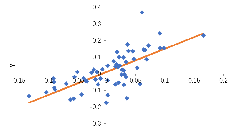
Figure 4: The correlation between Under Armor and the S&P 500 Index.

3.2. Correlation and Covariance Matrix Analysis

3.2.1. Analysis of Excess Return and Volatility

Figure 5 to Figure 8 depict the excess returns of stocks selected from the S&P 500 Index of Daily Consumption and Discretionary Stocks. According to the information in figures, it can finds that the volatility of optional consumption is greater than that of daily consumption [10].

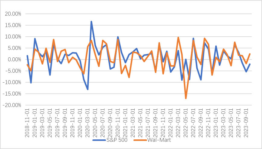
Figure 5: S&P500 and Walmart excess returns.

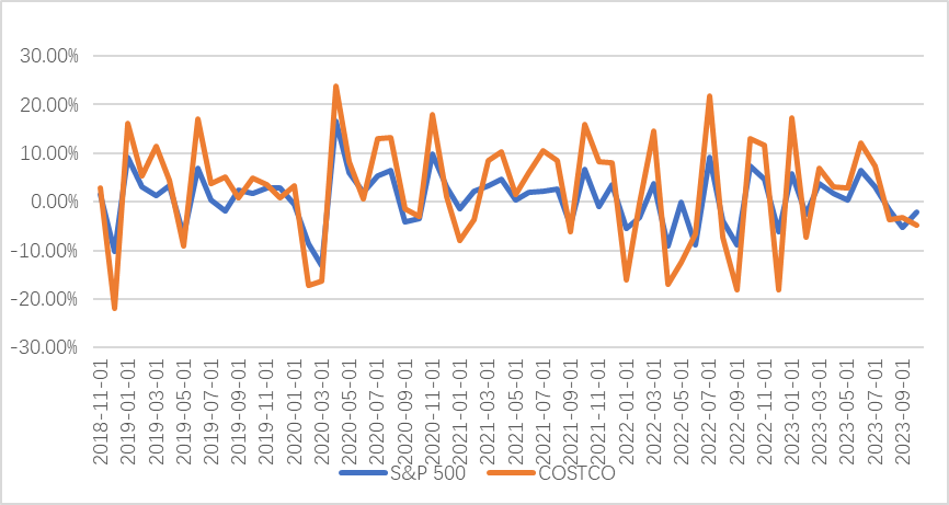
Figure 6: S&P500 and Costco excess returns.

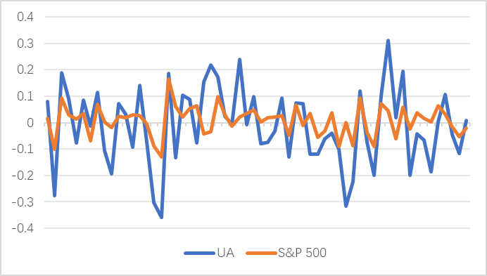
Figure 7: S&P500 and Under Armor excess returns.

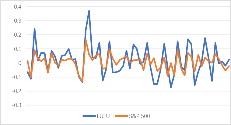
Figure 8: S&P500 and Lululemon excess returns.

3.2.2. Conclusion on the Optimal Investment Portfolio

Table 5 shows the estimates of risk parameters for the S&P index and four securities. The importance of diversification can be seen from the standard deviation of the residuals. The β value represents the sensitivity coefficient of each company to the market. The larger the β coefficient, the more sensitive it is to market changes. As can be seen from Table 5, the β value of the optional consumption industry is significantly higher than that of daily consumption and the S&P Index, and it is more sensitive to market changes. High sensitivity to changes.

Table 5: Global investable risk parameters (annual).

Table 6 shows the correlation matrix of excess return residuals from the regression of securities against the S&P Index. The shaded part shows the correlation of the same sector. Under normal circumstances, the cross-industry correlation is generally much smaller. In the table, the correlation coefficient between Costco and Walmart's residual value reaches 0.6354, which is a strong correlation. Due to the particularity of the discretionary consumer industry, which is affected by consumers' personal preferences and brand positioning characteristics, the residual value correlation coefficient between Under Armor and Lululemon is low.

Table 6: Residual value correlation coefficient.

Table 7 shows the co variances obtained by the single-index model. The variances of the S&P 500 index and individual stocks are located on the diagonal.

Table 7: Exponential covariance matrix.

Table 8 shows that the α of Costco, Walmart, and Lululemon are positive and higher than the S&P 500 index , indicating that the premium of these three stocks is higher than that of tracking the market index fluctuation trend, indicating that these three stocks are undervalued, investors will correspondingly increase their proportion in the risk portfolio when investing. On the contrary, if Under Armor's alpha value is negative, it means that the security is overvalued, and investors will reduce the weight when investing.

Table 8: Macro prediction and α value prediction.

Table 9 shows the calculation of the optimal risk portfolio. The final calculation results show that when the active portfolio composed of these four companies accounts for 132.31 % and risk-free securities account for -32.31%, that is, when shorting risk- free securities, the most risky portfolio can be achieved to achieve its Sharpe ratio maximum. Notice that each security in the active portfolio has the same label as α. When short selling is allowed, the positions of the aggressive combination are larger, so this is an aggressive combination.

Table 9: Calculation of optimal risk asset portfolio.

4. Conclusion

The application of the index model to portfolio analysis provides a framework for macro analysis and security analysis, which is essential for the efficiency of optimal portfolios. After the above data and research, the following conclusions can be drawn: First, according to data and analysis, the optional consumption industry is more subject to market fluctuations and more sensitive to the market than the daily consumption industry. Second, the active portfolio composed of Costco, Walmart, Lululemon, and Under Armour accounts for 132.31%, and the risk-free securities account for -32.31%, that is, when the risk-free securities are short, the optimal portfolio can be reached, and the Sharpe ratio of the portfolio is the largest.

However, there are still shortcomings in this study. Although the data from October 2018 to November 2023 are selected, the sample size is still relatively small for the study of this theory, which may bring errors due to the small data scale. In addition, due to the influence of the overall environment of the novel coronavirus epidemic, the overall economic situation in part of the time is bad, and the market economy environment is in a relatively extreme situation, resulting in extreme risks, which is difficult to reflect regularly through the data, and will also cause certain errors in the research results. In future follow-up studies, the index model can be modified based on volatility, or the multi-factor investment index model can be formed by adding factor variables to reduce errors.

References

[1]. Yan, H. B., & Meng, Y. (2024). Portfolio research based on ESG-CVaR model. Contemporary Economy, 41(01), 74-84.
[2]. Li, X., & Wang, B. (2020). Robust sharp single index model building and its comparative study. Journal of Mathematical Statistics and Management, 39(3), 544-555.
[3]. Liu, M. (2022). Analysis of Optimal Portfolio Value based on Single Index Model. China Prices, (10), 93-96.
[4]. Poornima, S., & Remesh, P. A. (2019). Optimal portfolio construction of selected stocks from NSE using Sharpe's single index model. International Journal of Management, IT and Engineering, 7(12), 283-298.
[5]. Al-Nassar, N. S., Yousaf, I., & Makram, B. (2023). Spillovers between positively and negatively affected service sectors from the COVID-19 health crisis: Implications for portfolio management. Pacific-Basin Finance Journal, 79, 102009.
[6]. Chen, Y., Zhao, J., Zuo, L., et al. (2021). Wealth Today (China Intellectual Property), (10), 49-51.
[7]. Micán Rincón, C. A., Rubiano-Ovalle, O., Delgado Hurtado, C., & Andrade-Eraso, C. A. (2023). Project portfolio risk management. Bibliometry and collaboration Scientometric domain analysis. Heliyon, 9(9), e19136.
[8]. Mahmud, I. (2019). Optimal Portfolio Construction: Application of Sharpe's Single-Index Model on Dhaka Stock Exchange. Jema: Jurnal Ilmiah Bidang Akuntansi dan Manajemen, 16(1), 60-92.
[9]. Sweetly, M. (2020). Portfolio optimization using the capital asset pricing model (CAPM) at the IDX-30 index company on the Indonesia stock exchange (IDX). International Journal of Management IT and Engineering, 10(11), 50-57.
[10]. Cheng, S. (2022). Correction en source model based on the volatility of the stock index strategy research, Shanghai University of Finance and Economics.
Cite this article
Xiao,L. (2024). Portfolio Management of Consumer Industry Based on Index Model. Advances in Economics, Management and Political Sciences,84,30-41.
Data availability
The datasets used and/or analyzed during the current study will be available from the authors upon reasonable request.
Disclaimer/Publisher's Note
The statements, opinions and data contained in all publications are solely those of the individual author(s) and contributor(s) and not of EWA Publishing and/or the editor(s). EWA Publishing and/or the editor(s) disclaim responsibility for any injury to people or property resulting from any ideas, methods, instructions or products referred to in the content.
About volume
Volume title: Proceedings of the 2nd International Conference on Management Research and Economic Development
© 2024 by the author(s). Licensee EWA Publishing, Oxford, UK. This article is an open access article distributed under the terms and
conditions of the Creative Commons Attribution (CC BY) license. Authors who
publish this series agree to the following terms:
1. Authors retain copyright and grant the series right of first publication with the work simultaneously licensed under a Creative Commons
Attribution License that allows others to share the work with an acknowledgment of the work's authorship and initial publication in this
series.
2. Authors are able to enter into separate, additional contractual arrangements for the non-exclusive distribution of the series's published
version of the work (e.g., post it to an institutional repository or publish it in a book), with an acknowledgment of its initial
publication in this series.
3. Authors are permitted and encouraged to post their work online (e.g., in institutional repositories or on their website) prior to and
during the submission process, as it can lead to productive exchanges, as well as earlier and greater citation of published work (See
Open access policy for details).