1.Introduction

In recent years, China's real estate sector has been the main force of China's economic development, but as housing prices have risen, the purchasing power of Chinese residents' houses has gradually declined. China's economy is also facing the recession risk and the stock market has lost its weighted stock. Because of this, the Chinese government has successively issued favorable policies for the real estate in 2022 and 2023, so that the real estate can survive the crisis, and also rescue China A-share market. The real estate sector is an important weighted stock in China's A-share market, and the quality of stocks in the real estate sector directly affects the changes in the index of China's A-share market. This paper quantifies the relationship between housing prices and the China A-share market index from the perspective of data, and analyzes the impact of the decline in housing prices on the Chinese A-share market, and whether the China A-share market can maintain the stability of the index in the case of falling housing prices.

From a theoretical point of view, the current research shows that the factors that cause the shock of China's stock market are independent of the fundamental information to a certain extent [1]. However, from the perspective of Chinese stock market investors, China's stock market has a large number of retail investors, but retail investors have a limited ability to gather information and can only collect fundamental information. So, another type of view believes that retail investors will pay too much attention to fundamental information and changes in the macroeconomic situation in order to obtain excess returns, so that in the face of information, they will be overconfident or extremely panicked, and make irrational transactions, resulting in violent shocks in the stock market[2][3]. At present, most of the research focuses on the changes in the volatility of the stock market itself, and does not combine the changes in China's real estate industry with stock volatility. This article will further explain the impact of the real estate industry downturn on the stock market in the future under the circumstance that macro information has an impact on the stock market shock.

We add to the literature by using Monte Carlo algorithm and the Monte Carlo algorithm is used, with reference to Kaczmarzyk Jan's Forecasting currency risk of enterprise's asset portfolio using the Monte Carlo The Monte Carlo algorithm used in the simulation, and the index volatility and annual growth rate of the China CSI Index 300 were used as the original parameters. The simulation is carried out and the paper analyzes the future development of the real estate industry.[4]

2.Empirical analysis and discussion

2.1.Research hypothesis

Due to the large number of real-world factors, the algorithms and variables used in this question cannot fully cover all the variables. So, some subjective assumptions are required. In order to facilitate analysis, this paper has the following assumptions:

1.The fluctuation of housing price will have an impact on the performance of real estate companies.

2.The poor performance of real estate companies will cause stock prices to fall.

3.The fluctuation of housing price will lead to the fluctuation of stock index.

2.2.Data description

The China’s Shanghai and Shenzhen 300 index (CSI Index 300) is made of the most liquid stocks in the Shanghai and Shenzhen stock exchanges. Since China's Shanghai and Shenzhen 300 index contains many listed companies, there are too many factors to shock and cannot clearly reflect the downward trend of the real estate industry, and how much impact it has on China's stock market. So, the CSI 300 index can be selected to show the results more intuitively[5].

First, the national average housing price from 2007 to 2022 was collected from the National Bureau of Statistics of China. The survey method of house price: the new residential sales price survey is a comprehensive survey, and the basic data is directly used for local housing registration data of real estate authorities. The second-hand housing sales price survey is not a comprehensive survey and typical survey, and collects basic data according to the combination of reporting by real estate agencies or housing service platforms, providing by real estate authorities and purchasing prices by investigators on the spot. The annual average of China's CSI 300 index was collected from the National Bureau of Statistics of China and descriptive statistics were made and curves were plotted.

Figure 1: Data scatter diagram

It can be seen from the figure that China's housing prices rose steadily before 2021. After 2021, due to the slowdown in China's economic growth, the decline in people's spending power, and the excessive debt of some Chinese real estate companies, the performance of thunderous performance and other factors, the sales of residential houses will decrease after 2021.

In 2007, the CSI 300 index reached its peak for the first time, but affected by the 2008 financial crisis. In 2008, the CSI 300 index fell sharply. After the national policy macro control, the CSI 300 index rose steadily. But due to the performance of the real estate industry after 2021, there was a downward trend.

Table 1: Descriptive statistics

2.3.Establish a regression model

Firstly, the correlation between housing prices and the CSI 300 Index is analyzed, and the purpose of correlation analysis is to study the strength of the linear correlation between the two variables through sample data.

As can be seen from the Figure 1, there may be an linear relationship between housing prices and the CSI 300 index.

After that, the correlation coefficient is calculated, and the Spearman correlation coefficient is used in this paper. The Spearman correlation coefficient is calculated by using matrix rank. If the house prices are correlated with the index, the corresponding rank\( {U_{i}} \)and\( {V_{i}} \)will be also synchronized.

After obtaining\( {U_{i}} \)and\( {V_{i}} \), the\( D_{i}^{2} \)statistic is calculated. If there is a strong positive correlation between the two variables,\( D_{i}^{2} \)should be small, and the order correlation coefficient should be larger. If there is a strong negative correlation between the two variables, then\( D_{i}^{2} \)should be larger, and the order correlation coefficient should be negative, and the absolute value should be larger. Formula for calculating Spearman's correlation coefficient:

\( \sum _{i=1}^{n}D_{i}^{2}=\sum _{i=1}^{n}{({U_{i}}-{V_{i}})^{2}} \)(1)

\( R=1-\frac{6\sum D_{i}^{2}}{n({n^{2}}-1)} \)(2)

After the correlation coefficient is calculated, the correlation coefficient test was carried out to statistically inference whether the two variables came from the population were correlated.

Null hypothesis: H₀: there is correlation between house prices and the CSI 300.

Alternative hypothesis: H₁: there is no correlation between house prices and the CSI 300.

Construct the Spearman coefficient statistic:\( Z \)=\( R\sqrt[]{n-1} \), and cipher out the corresponding\( P \)value. The significant intervals selected in this paper are:\( α=5\% \)｡

If\( P≤α \), then the null hypothesis is rejected, there is a linear correlation between the two populations.

If\( P≥α \), the null hypothesis isn’t rejected refuse, there is no linear correlation between the two populations.

The correlation analysis was carried out using SPSS software, and the results were as follows:

Table 2: Spearman correlation analysis

P: 0.006\( ≤0.05 \), So reject the null hypothesis H₀, and there is a correlation between house prices and indices.

Then, the sample data is used to establish a regression model, which can be analyzed from the scatter plot, and the house price and index meet the polynomial regression([6]). In economic research, the stock price of real estate industry has a great relationship with the fluctuation of housing price. The stock price of real estate industry will also affect the CSI 300 index. So, the principle of polynomial regression: housing price is independent variable, CSI 300 index is dependent variable([7]).

Suppose the regression equation is:

y=\( {β_{0}}+{β_{1}}x+{β_{2}}{x^{2}}+{β_{3}}{x^{3}}+∙∙∙∙+{β_{n}}{x^{n}} \)(3)

\( {β_{0}}={β_{0}}-μ\sum _{i=1}^{n}({f_{β}}({x^{(i)}})-{y^{(i)}}) \)(4)

\( {β_{1}}:={β_{1}}-μ\sum _{i=1}^{n}({f_{β}}({x^{(i)}})-{y^{(i)}}){x^{(i)}} \)(5)

\( {β_{2}}:={β_{2}}-μ\sum _{i=1}^{n}({f_{β}}({x^{(i)}})-{y^{(i)}}){x^{{(i)^{2}}}} \)(6)

\( ⋯⋯ \)

\( { β_{n}}:={β_{n}}-μ\sum _{i=1}^{n}({f_{β}}({x^{(i)}})-{y^{(i)}}){x^{{(i)^{n}}}} \)(7)

So, the fitted image is:

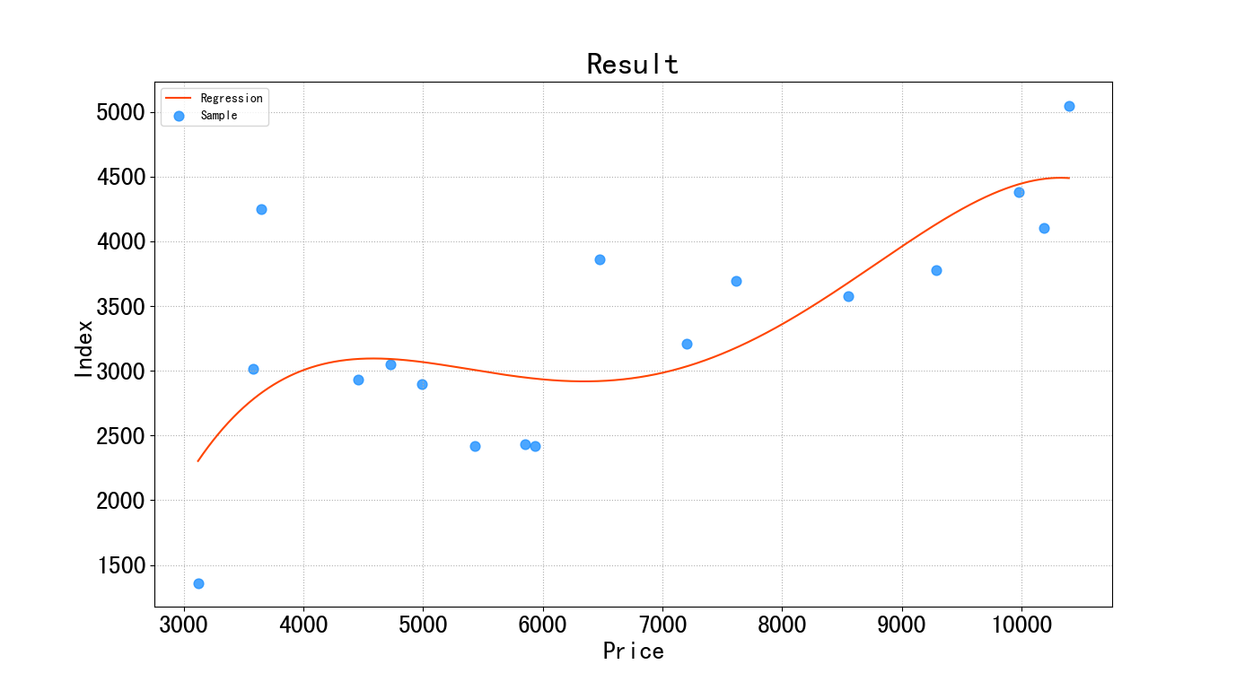
Figure 2: Forecast result

The equation after regression fitting is:

\( y=-15162.51+11.98{x^{1}}-0.00283{x^{2}}+2.83×{10^{-7}}{x^{3}}-9.98×{10^{-12}}{x^{4}} \)(8)

The goodness of fit of the regression equation R²=0.5648. This suggests that when the prices are changed, it will explain 56.48% of the change in the index.

2.4.Time series forecasting

In order to analyze house prices in the next few years, this paper uses a time series algorithm to analyze house prices.

First of all, it is necessary to determine whether China's housing prices are suitable for the time series algorithm, that is, whether the sample data is stationary series, and if it is a non-stationary series, it needs to be converted into a stationary series to be analyzed.

The ADF test begins with a hypothesis test:

H₀:There are unit roots, and the sequence is not stationary.

H₁:There is no unit root, and the sequence is smooth.

If the resulting significance test statistic is less than the confidence level (1%, 5%, 10%), the null hypothesis can be rejected, otherwise the null hypothesis is accepted.

Then, the original data is tested, and the autoregressive equation of the model is:

\( y=c+βt+α{y_{t-1}}+{e_{t}} \)(9)

\( {Y_{t}} \)is the value of the time series at time t.\( {y_{t-1}} \)is a lag of 1 unit for the time series and\( {X_{e}} \)is an exogenous variable.

After testing, the results are as follows:

Table 3: ADF statistic

The ADF test statistics are all greater than the critical values of 1%, 5% and 10% statistics, and the P values are all greater than 1%, 5% and 10% confidence levels, so the original data is not a stationary series and needs to be differentially processed on the original data.

The first-order difference calculation method is to subtract the lag value of the variable\( {x_{t}} \)from the current value to obtain a new sequence, for the random process\( {x_{t}} \). The first-order difference formula is:

\( { D_{{x_{t}}}}={x_{t}}-{Lx_{t-1}}=(1-L){x_{i}} \)(10)

D is called the first-order difference operator, and L is the lag operator.

The autoregressive equation of the model after difference is:

\( y=c+βt+α{y_{t-1}}+{φ_{1}}∆{Y_{t-1}}+{φ_{2}}∆{Y_{t-2}}+⋯+{φ_{p}}∆{Y_{t-p}}+{e_{t}} \)(11)

The ADF test after the difference is:

Table 4: ADF statistic

As can be seen from the table 4, the ADF test statistic is less than -2.749 and the P value is less than 0.05. So, the null hypothesis is rejected and the differential series is stationary. After that, the autocorrelation coefficient (ACF) and partial autocorrelation coefficient (PACF) are calculated.

The principle of calculating autocorrelation function and partial autocorrelation function:

The autocorrelation coefficient is defined as:

\( {ρ_{k}}=\frac{Cov({x_{t}},{x_{t+k}})}{\sqrt[]{Var({x_{t}})}\sqrt[]{Var({x_{t+k}})}} \)=\( \frac{E({x_{t}}-μ)({x_{t+k}}-μ)}{\sqrt[]{E[{({x_{t}}-μ)^{2}}]}\sqrt[]{E[{({x_{t+k}}-μ)^{2}}]}} \)(12)

\( {ρ_{k}} \)is no unit of measurement.

Because for a smooth process satisfies:\( Var({x_{t}})=Var({x_{t+k}})=σ_{x}^{2} \),Therefore, the autocorrelation coefficient formula can be rewritten as:

\( {ρ_{k}}=\frac{Cov({x_{t}},{x_{t+k}})}{σ_{x}^{2}}=\frac{{γ_{k}}}{σ_{x}^{2}} \)(13)

Because\( {γ_{0}}=σ_{x}^{2} \),The autocorrelation coefficient can be expressed as:

\( {ρ_{k}}=\frac{{γ_{k}}}{{γ_{0}}} \)(14)

When k is zero,\( {ρ_{0}} is one \).

Because the autocorrelation function is symmetrical with k=0, when studying house price data, you only need to analyze the positive half of the autocorrelation function. In this paper\( {ρ_{k}}={ρ_{-k}} \), the ARIMA time series model is used, and the autocorrelation coefficient image shows a tailing trend.

The partial autocorrelation coefficient is another way to describe the structural characteristics of stochastic processes, and the k-order autoregressive model is expressed as follows:

\( {x_{t}}={∅_{k1}}{x_{t-1}}+{∅_{k2}}{x_{t-2}}+⋯+{∅_{kk}}{x_{t-k}}+{u_{t}} \)(15)

\( {∅_{kk}} \)is the last regression coefficient.

Then, the partial autocorrelation function is calculated using the autocorrelation function as follows:

\( {ρ_{t}}={∅_{k1}}{ρ_{j-1}}+{∅_{k2}}{ρ_{j-2}}+⋯+{∅_{kk}}{ρ_{j-k}} \)(16)

j=1,2,3,…,k

\( {ρ_{t}} \)and\( {∅_{kj}} \)are vector quantity.

Replace k = 1, 2, 3 ,...substituting the above equation for continuous solving. The partial autocorrelation function can be obtained. The partial autocorrelation coefficient image has a tailing trend in the ARIMA model

The first-order differential ACF and PACF images are as follows:

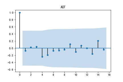
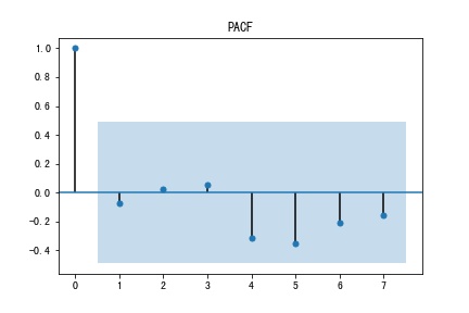
Figure 3: ACF Figure 4: PACF

It can be seen from the two figures that autoregressive(p) is zero and moving average(q) is zero. Then, the q*p model fitting was carried out, and the values of AIC and BIC were compared with the results of model fitting. The smaller the value of BIC, the better the fitting degree of the model, and finally the optimal model was found. Then the order of the model fitting was used as the order of the final fit. The final model of ARIMA was obtained as ARIMA (0,1,0).

Then, the model parameter test and the model significance test were carried out.

Parameter test of the model: check whether each unknown parameter is significantly 0, and check whether the model is the most streamlined. If the parameter is not significant and non-zero, it can be eliminated from the fitting model.

Model significance test: the white noise test of the residuals. If the residuals are white noise sequences, the original sequence information will be fully extracted, and the LB statistic is calculated. If the P value is less than 0.05, it is a non-white noise sequence. If the P value is greater than 0.05, it means that the residuals are white noise sequences

The results of the test are as follows:

Table 5: Model determination

Table 6: Model

Because the P>|z| of the each parameter is less than 0.05, the null hypothesis is rejected. The model parameter test effect is significantly non-0, and the model is the most concise model.

The white noise of the differential sequence is:

Table 7: White noise test results of difference

As can be seen from the table, at Q1, the P value is already greater than 0.05, which is not significant, and the assumption that the residual of the model is a white noise sequence cannot be rejected.

Then the residual analysis of the model is carried out according to the following principle:

\( {δ_{i}}={y_{i}}-{θ_{i}} \)(17)

\( {δ_{i}} \)is the residual,\( {y_{i}} \)is the true value,\( {θ_{i}} \)is the predicted value.

The analysis results are as follows:

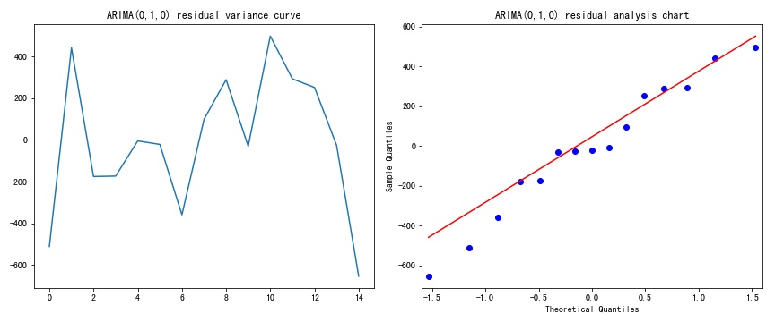
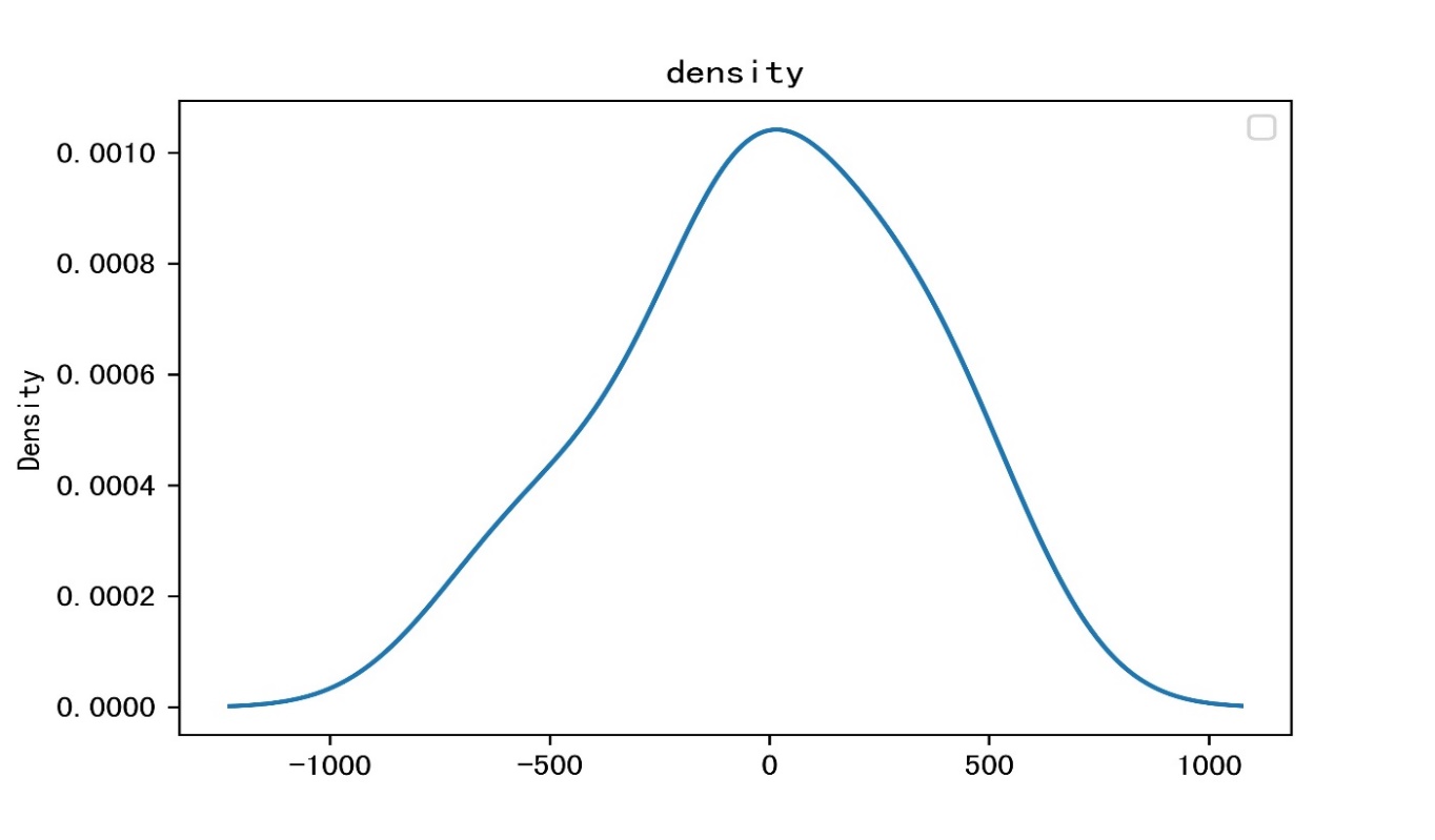
Figure 5: Residual analysis

In the Q-Q diagram of residuals, the horizontal axis is the theoretical quantile, and the vertical axis is the sample quantile. As can be seen from the figure, the data points are distributed along a straight line, indicating that the residual value conforms to the normal distribution.

To sum up, the house prices is predicted by the ARIMA (0,1,0) model. The formula is as follows:

\( {x_{t}}={x_{t-1}}+{ε_{t}} \)(18)

The predictions are as follows:

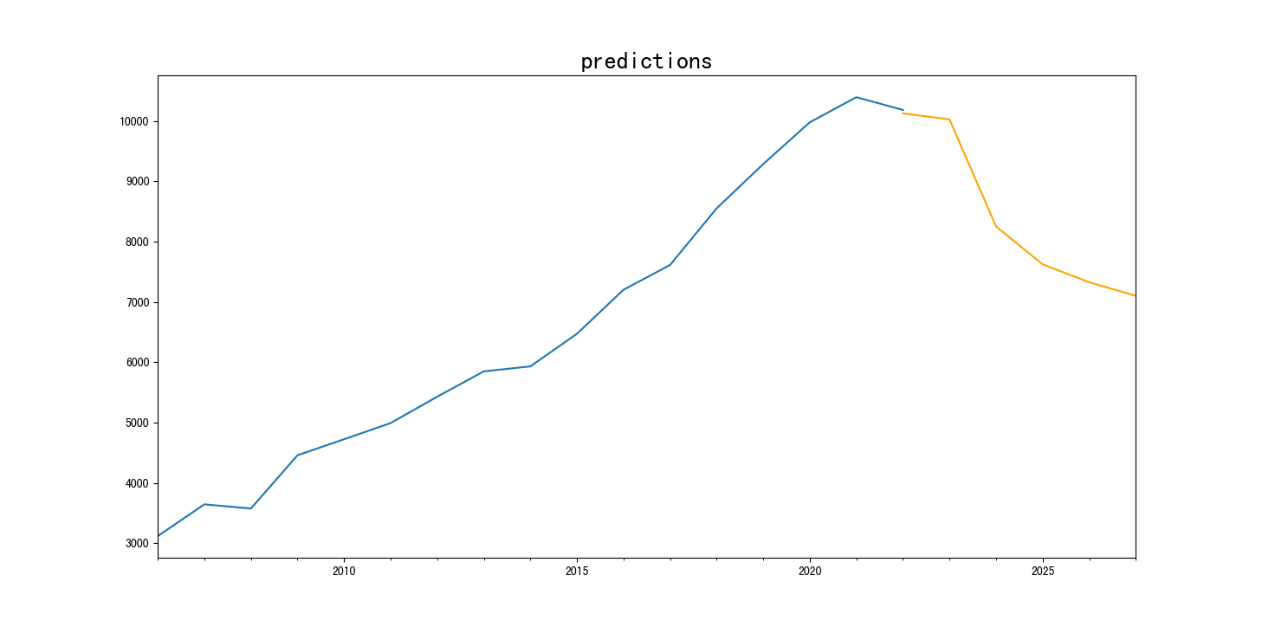
Figure 6: Time series prediction

The predicted values are:

Table 8: Forecast result

2.5.Forecast the CSI index

Then, the change of the CSI 300 Index from 2023 to 2027 is calculated by fitting the curve between house prices and the index. Here are the results:

Figure 7: Forecast result

Table 9: Forecast result

2.6.Long-term simulation of Monte Carlo algorithm

To calculate the index volatility, the formula used in this paper is as follows:

\( σ=\sqrt[]{\frac{\sum _{i=1}^{N}{({x_{i}}-x)^{2}}}{N}} \)(19)

\( s=\frac{\sum _{i=1}^{N}{x_{i}}}{N} \)(20)

\( ε=\frac{σ}{s} \)(21)

Among them,\( σ \)is the standard deviation,\( s \)is the average of the CSI 300 index, x is the CSI 300 index, and\( ε \)is the volatility of the CSI 300 index.

This results in a volatility of 0.248678. The growth rate of the CSI index is then calculated, and the calculation formula is as follows:

\( GR=\frac{{x_{i+1}}-{x_{i}}}{{x_{i}}} \)(22)

Among them, x is the CSI index, GR is the annual growth rate, and the calculated result is 0.09927.

Then I use the Monte Carlo algorithm to analyze the Shanghai and Shenzhen indexes in a long-term stable state. Simulation of changes in the CSI and Shenzhen indices is carried out to observe the specific impact of the CSI 300 Index and the final stable state when the housing prices fluctuates violently.

In this paper, the average annual growth rate and volatility of the index are used to calculate the average annual return. The index is calculated from the average annual return, and in the same way, it is simulated 1000 times, which is delayed by 24 years. Finally, the average value is obtained. The specific analysis process is as follows:

First, by using the software to conduct 1,000 simulations, it can be concluded that the Shanghai and Shenzhen indices will show a downward trend in the future.

The difference in extreme values is 6000. The final distribution of the simulation results is as follows:

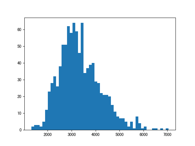
Figure 8: The final distribution

By seeing from the distribution map, the final average value is 3316.48. When house prices are volatile, China's CSI 300 index will stabilize at 3316.48, which returns to the index state of 2016.

3.Further analysis

Because China is socialist country and the Chinese government has the ability to regulate and control the economy in a unified manner. In order to further study the shock of housing prices, it is necessary to add the government factor to the model. So, the China Economic Uncertainty Index (CEPUI) is used. The China Economic Uncertainty Index is a measure of China's economic policy uncertainty, which is based on a methodology developed by Baker, Bloom, and Davis.[8] This method is an indicator constructed using a variety of information sources. The China Economic Policy Uncertainty Index is calculated as the sum of three components: the frequency of news articles that contain words related to economic policy uncertainty, the proportion of those articles that also mention the economy or specific policy areas, and the degree of divergence among economic forecasters on the future path of economic policy uncertainty on key economic variables. A higher CEPUI value indicates higher economic policy uncertainty. According to the method of Davis et al., this paper uses the economic policy uncertainty index to comprehensively measure economic policy uncertainty and plot it into a line chart.

Figure 9: CEPUI

From the line chart, it can be seen that before 2001, China's economic policy uncertainty has been at a low level, until after joining the WTO in 2001, China's uncertainty has risen slightly. In 2008 during the global financial crisis, the index showed a significant rise, which is close to the high point of 200. With the trend of trade globalization, China's economic policy is more uncertain. From 2010 to 2013 European sovereign debt crisis, China's economy turned into a new stage of medium and high-speed growth, some domestic economists have concerns about the future of China's economic development. In 2013, the Chinese government proposed the Belt and Road Initiative, which will unite countries around the world to jointly develop the economy, and China's economic policy has a specific general direction. So, the uncertainty is reduced, and the index is stable at about 100. In 2017, the United States withdrew from the Trans-Pacific Partnership (TPP), raising the risk of future economic uncertainty in China. In 2018, the United States imposed a series of trade sanctions on China, which caused a serious impact on China's economy. At the end of 2019, the new crown epidemic broke out, and the future economy was even more uncertain, until the end of 2022 and the beginning of 2023, when the epidemic ended, the global economy recovered. The economic trend improved, and the risk of uncertainty was reduced.

The uncertainty index is now added to the time series, as the government's influencing factor. When the uncertainty index is lower, the government's policy will be looser, and the higher the uncertainty index, the government's policy will be greater to promote economic development.[9] Then, through the curve fitting equation of housing prices and the index, the changes of the CSI 300 index from 2023 to 2027 under the macroeconomic control of the Chinese government are calculated. When the government factor is added, the image of the forecast is:

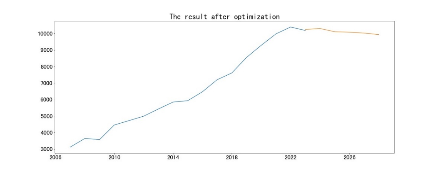
Figure 10: Revised result

The predicted results are:

Table 10: Forecast result

From the analysis of the above methods, under the government's macroeconomic control, from 2023 to 2027, the CSI 300 index will decline slightly less and will not form a violent shock.

4.Conclusions and Implications

4.1.Conclusions

Through theoretical research and empirical analysis, this paper uses polynomial regression to analyze the equation relationship between China's housing prices and the CSI 300 index, and uses time series to predict the changes of the CSI 300 index from 2023 to 2027 without government macroeconomic control, and the changes of the CSI 300 index from 2023 to 2027 under the government's macroeconomic control. Based on the above analysis, the following conclusions are made:

Firstly, without the government's macroeconomic control, housing prices will fall sharply and produce a herd effect, which may make housing prices enter a downturn in the short term. The CSI 300 index will fluctuate violently with housing prices and resulting in a serious decline. In the long run, it will tend to be around 3300 points, and eventually return to the index state in 2016, which will have a violent impact on China's stock market, which may cause a large number of investors to lose confidence in China, the rapid withdrawal of funds, and the further decline of the index, resulting in irreparable

Secondly, from a practical point of view, the Chinese government will make corresponding adjustments to housing prices and China's financial market, after taking into account the government's macroeconomic control. Although housing prices will fall, but it will fall steadily, which is a normal market cycle, and the CSI 300 index changes little, which can be regarded as a normal fluctuation of the stock market. It can be further analyzed that the Chinese government plays a key role in the macroeconomic regulation and control of the economy and the supervision of the financial market, and the Chinese government is an important factor that cannot be ignored in the analysis of China's financial market.

4.2.Research implications

The stock market is an important part of China's financial market. The fluctuation of the stock index is the reflection of the development of the companies. When an industry is developing poorly, investors will sell the shares of companies which are in this industry. So, in the face of the trend of falling housing prices in China, retail investors have lost confidence in real estate companies, and will have panic. This will result in the continuous decline in the stock price of the real estate industry, which will eventually affect the upside of the Shanghai and Shenzhen indexes, and further make a large number of retail investors bearish on the Shanghai Composite Index, which has a serious impact on China's financial market. But due to the macro control of the Chinese government, China's housing prices will be steady and there will be no sharp decline

At the same time, in order to maintain the stable development of China's economy, the Chinese central government will encourage people to invest in real estate and buy residences.

References

[1]. Li Bolong. Sparse Component and Stock Market Volatility Prediction in Macro Fundamentals[J].Operations Research and Management,2023,32(09):186-192
[2]. Xu Jing. Research on the influence and prediction of investors' macroeconomic attention on stock price fluctuations[D].Nanjing University of Information Science and Technology, 2023.DOI:10.27248/d.cnki.gnjqc.202 3.000637
[3]. G. T B ,Doruk A G ,Thomas J , et al.Do the rich gamble in the stock market? Low risk anomalies and wealthy households[J].Journal of Financial Economics,2023,150(2):
[4]. Zhou Shuang, Liu Yun. Analysis of the current situation and prospect of real estate in China[J].Time-honored brand marketing,2023(20):67-69.
[5]. Hong K B ,Warren B ,Jisok K .Why is stock market concentration bad for the economy?[J].Journal of Financial Economics,2021,140(2):
[6]. Lie, Huang Yufang, Tan Meifang, etc.The change of individual stock curve and the regression of its opening price-Markov prediction[J].Contemporary education theory and practice,2011,3(11):132-134
[7]. Wan Yiyi. An empirical analysis of the interaction mechanism between China's real estate market and stock market[D].Jiangxi University of Finance and Economics,2014..
[8]. Bagh T ,Waheed A ,Khan A M , et al.Effect of Economic Policy Uncertainty on China’s Stock Price Index: A Comprehensive Analysis Using Wavelet Coherence Approach[J].SAGE Open,2023,13(4):
[9]. Peng Jiamin. The impact of economic policy uncertainty on macroeconomic cycle[D].Guangdong University of Finance and Economics,2023.DOI:10.27734/d.cnki.ggdsx.2023.000521.
Cite this article
Liu,J. (2024). The Impact of the Real Estate Recession on China's Stock Market. Advances in Economics, Management and Political Sciences,84,258-272.
Data availability
The datasets used and/or analyzed during the current study will be available from the authors upon reasonable request.
Disclaimer/Publisher's Note
The statements, opinions and data contained in all publications are solely those of the individual author(s) and contributor(s) and not of EWA Publishing and/or the editor(s). EWA Publishing and/or the editor(s) disclaim responsibility for any injury to people or property resulting from any ideas, methods, instructions or products referred to in the content.
About volume
Volume title: Proceedings of the 2nd International Conference on Management Research and Economic Development
© 2024 by the author(s). Licensee EWA Publishing, Oxford, UK. This article is an open access article distributed under the terms and
conditions of the Creative Commons Attribution (CC BY) license. Authors who
publish this series agree to the following terms:
1. Authors retain copyright and grant the series right of first publication with the work simultaneously licensed under a Creative Commons
Attribution License that allows others to share the work with an acknowledgment of the work's authorship and initial publication in this
series.
2. Authors are able to enter into separate, additional contractual arrangements for the non-exclusive distribution of the series's published
version of the work (e.g., post it to an institutional repository or publish it in a book), with an acknowledgment of its initial
publication in this series.
3. Authors are permitted and encouraged to post their work online (e.g., in institutional repositories or on their website) prior to and
during the submission process, as it can lead to productive exchanges, as well as earlier and greater citation of published work (See
Open access policy for details).