1. Introduction

The rapid development of China's market economy has significantly enhanced the global inter-connectivity of the world economy, paralleled by considerable growth and expansion within the Chinese stock market. Since its establishment in 1986, China's stock market has witnessed steady growth and moderation, marked by a pivotal moment in December 1990 with the founding of the Shenzhen and Shanghai Stock Exchanges. Despite these advancements, the Chinese stock market lacks a well-developed supply and demand system and a robust market monitoring mechanism, attributable to its relatively brief history and sluggish developmental pace. Early in its evolution, the market encountered numerous challenges, further complicated by the uncertainties associated with China's ongoing economic transition and globalization. These factors indicate that the Chinese stock market is still in the nascent stages of its development, characterized by its fundamental growth, development, and standardization processes [1].

Time series analysis, a pivotal statistical technique for processing dynamic data, holds an indispensable role in financial research. Its theoretical foundations and methodological approaches are crucial for analyzing financial time series [2]. Various models, consisting of the Auto-regressive Conditional Heteroskedastic (ARCH) model, Generalized-ARCH (GARCH) model, and Auto-regressive Moving Average (ARMA) model, have significantly contributed to the forecasting of financial time series. Notably, the GARCH model, which is an expansion of Engle's ARCH model, is extensively utilized to study the characteristics and patterns of financial data. The choice of GARCH specification influences the modeling outcomes, necessitating the selection of the most suitable GARCH variant for accurate modeling. This entails exploring an appropriate residual distribution to effectively describe and predict trends in China's stock market, as well as to analyze and elucidate the relationship between Shanghai and Shenzhen’s stock markets [3].

2. Materials and Methods

2.1. Shanghai (securities) Composite Index

The Shanghai Stock Exchange Composite Index, also known as the Shanghai Composite Index, serves as a pivotal stock index of the Shanghai Stock Exchange. It is instrumental in reflecting the comprehensive performance of the stock market associated with this exchange. This index provides a broad picture of stock price performance within the Shanghai securities market since it encompasses all listed stocks on the Shanghai Stock Exchange, including both A shares and B shares.

The methodology employed for calculating the Shanghai Composite Index involves a total equity weighting approach. This calculation is the aggregate of the products of individual stock prices and their respective issued shares. Officially inaugurated on July 15, 1991, the index utilizes December 19, 1990, as its base period with an initial benchmark of 100 points.

Fluctuations in the Shanghai Composite Index are indicative of the overarching stock price movements on the Shanghai Stock Exchange. An increase in the index suggests a general rise in stock prices across the exchange, whereas a decline indicates a widespread drop in stock values [4].

As a critical barometer of China's stock market health, the Shanghai Composite Index garners significant attention from investors, financial analysts, and the media alike. Observations of its trends and modifications provide vital insights into the overall condition and trajectory of the Chinese stock market, facilitating evaluations and forecasts concerning economic development and the investment climate.

2.2. Shenzhen Component Index

The primary stock index of the Shenzhen Stock Exchange is the SZSE Component Index. It employs the amount of free-floating shares of the sample stocks as weights and the Pais weighting method to create a stock price indicator. It chooses 500 representative listed firms as sample stocks based on predetermined criteria. Using July 20, 1994, as the starting point, 1,000 points make up the base period.

2.3. The definition and the formula of stock return

Stock return refers to the profit or loss on an investment in a particular stock over a certain period of time. It's calculated as the percentage change in the price of the stock over that period, adjusted for any dividends received.

The formula to calculate stock return is:

\( Stock Return(\%)=(\frac{Current Price-Initial Price+Individuals}{Initial Price})×100 \) (1)

Where:

Current Price: The price of the stock at the end of the period.

Initial Price: The price of the stock at the beginning of the period.

Dividends: Any dividends received during the period.

2.4. The definition of logarithm return

The percentage change in an asset's value over time can be calculated using logarithm returns. Log returns, in contrast to simple returns, indicate the relative change in an asset's value as opposed to the absolute change.

The formula for calculating logarithmic returns is:

\( r=ln(\frac{{P_{t}}}{{P_{t-1}}}) \) (2)

3. Stock trend research and introduction of Garch model

3.1. Fluctuation characteristics of data

Table 1: stock data of SZSE Component Index in January 2012

Table 2: stock data of SSE Composite Index in January 2012

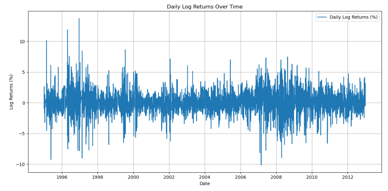
Figure 1: Logarithmic return rate of SZSE Component Index from 1995 to 2012

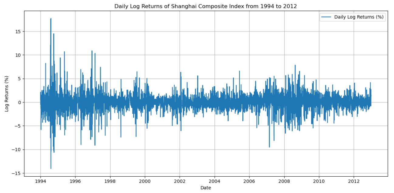
Figure 2: Logarithmic return rate of SSE Composite Index from 1994 to 2012

Table 1 and 2 represents detailed daily records of stock market activity for a series of trading days in January 2012. Each entry comprising several key variables: Date, which specifies the day of data collection; Open, the opening price of the market index; Highest, the peak value achieved during the trading day; Close, the closing value of the index; Lowest, the minimum value the index fell to; Amount (share), the total volume of shares traded, reflecting market activity; and Sum (yuan), which represents the total monetary value of trades conducted, expressed in yuan. These variables collectively provide a multifaceted view of daily market performance, crucial for analyzing market trends, liquidity, and economic impact during the specified period.

As depicted in Figures 1 and 2, the logarithmic returns of the Shanghai Composite Index and the Shenzhen Composite Index oscillate around the zero line, with variations ranging from -0.1 to 0.1, indicating stability within the expected bounds. Notably, during the period of 1995-1996, there were exceptional instances where fluctuations surpassed the 10% daily limit imposed by China's stock market regulations. These figures reveal a multi-peaked distribution of returns, suggesting significant volatility and illustrating the unpredictability of stock market returns. Furthermore, both the Shanghai Composite Index and the Shenzhen Stock Exchange Component Index exhibit clustering of fluctuations, a characteristic phenomenon in financial time series, where one period of intense market activity tends to precipitate another.

Table 3: Basic statistical properties of log returns of SSE and SZSE Composite Index

Table 3 provides an intuitive visualization of the normality of the logarithmic returns of the Shanghai Stock Exchange Composite Index and the Shenzhen Stock Exchange Component Index. Both indices exhibit negative skewness, suggesting an imbalance in their distributions, with most trading days yielding returns below their respective averages. A P-value of zero for both indices confirms their deviation from normal distribution.

The kurtosis values for both the Shanghai and Shenzhen indices exceed 3, indicating leptokurtic distributions characterized by pronounced peaks and heavy tails. Additionally, the mean value of the Shenzhen Component Index surpasses that of the Shanghai Composite Index. However, both indices have positive mean values, reflecting China's robust economic growth in recent years.

The standard deviation, a measure of volatility, shows that the Shenzhen Component Index is marginally more volatile than the Shanghai Composite Index by a difference of 0.02. This slight discrepancy suggests a somewhat greater volatility in the Shenzhen market, although the relatively low standard deviations of both indices indicate that China's stock market is still in stages of development and maturation.

3.2. Garch model fit

Use the Arch Test function to test whether the Shanghai Composite Index sequence has heteroskedasticity effects, then Use the arch_model function in python and student-t distribution to fit the GARCH model yields the following results:

Figure 3: test data of SSE Composite Index

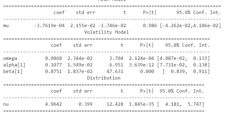
Figure 4: test data of SZSE Composite Index

From the obtained computational outcomes in figure 3 and figure 4, it is evident that all coefficients possess statistical significance, which underscores the influence of historical volatilities in the returns of the Shanghai Composite Index on current metrics. Notably, the phenomenon of volatility clustering remains pronounced. Moreover, the summation of α1 and β1 approximates to 1, suggesting that the sequence of conditional heteroskedasticity exhibits long memory. This implies a high persistence in yield fluctuations, robust speculative activities, and associated risks. Subsequent to the application of the GARCH model, an analysis of the residuals derived from the model's results can be conducted [5].

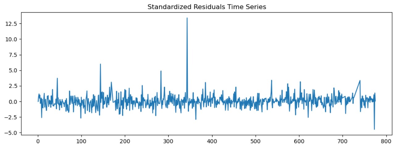
Figure 5: Standardized Residuals Time Series of SSE Composite Index

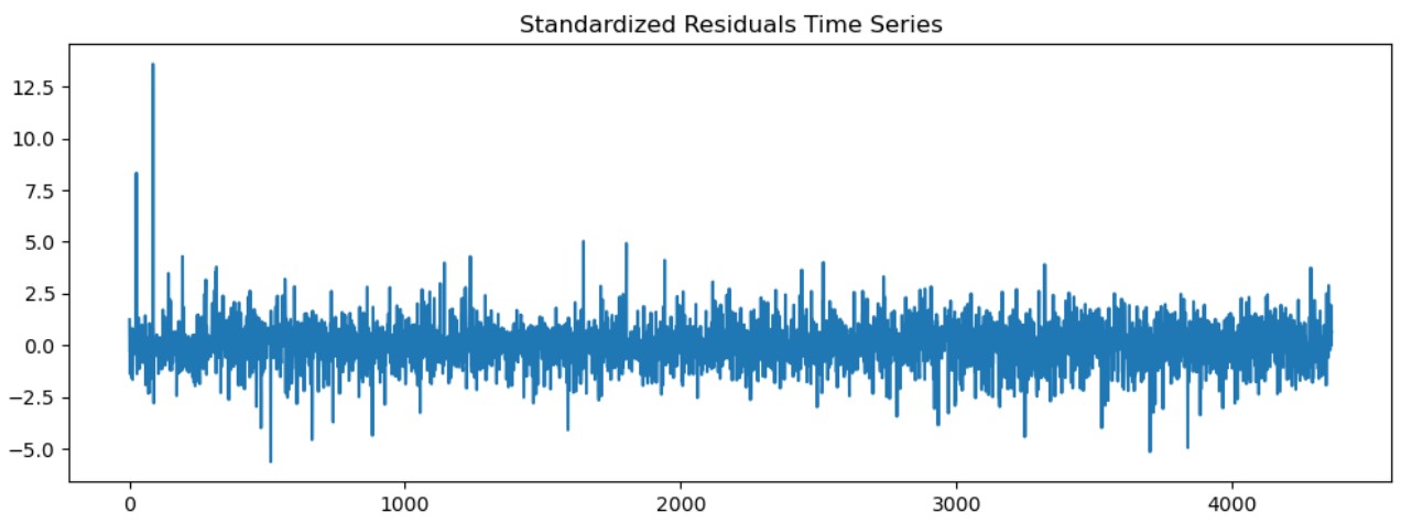
Figure 6: Standardized Residuals Time Series of SZSE Component Index

As shown in figures 5 and 6 are time series diagrams of the standardized residual sequence. It can be seen that the residual sequence has no obvious fluctuation aggregation effect.

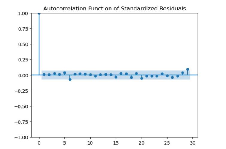
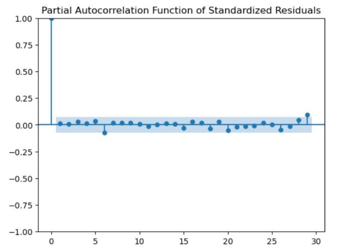
Figure 7: (Partial) Auto-correlation Function of Standardized Residuals of SSE Composite Index

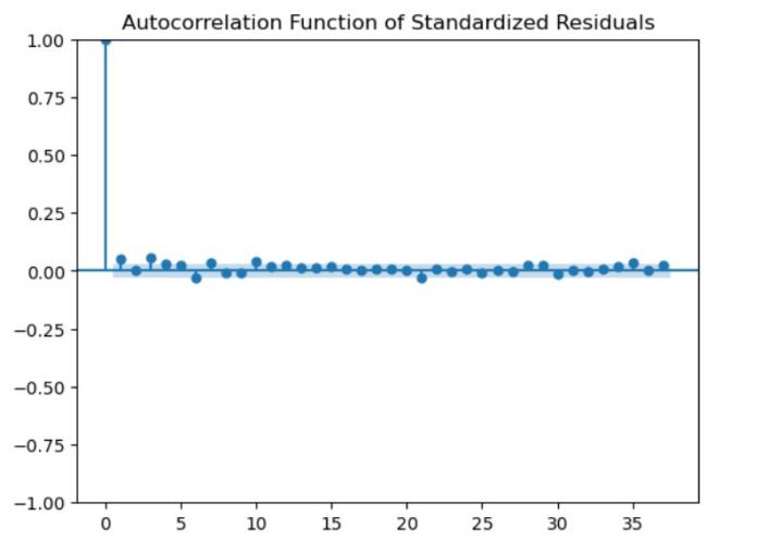
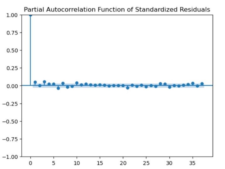
Figure 8: (Partial) Auto-correlation Function of Standardized Residuals of SZSE Component Index

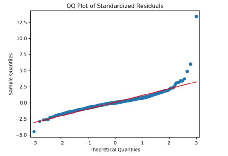
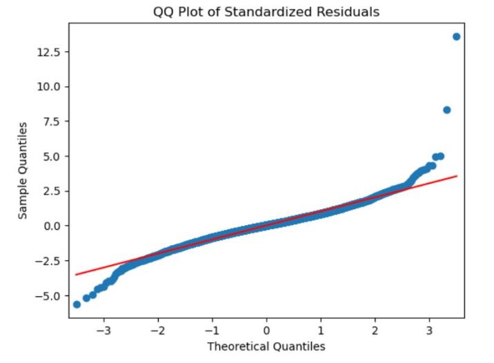
Figure 9: QQ plot of Standardized Residuals Figure 10: QQ plot of Standardized Residuals

Of SSE Component Index SZSE Component Index

Generating the Arch-Test function to evaluate the presence of heteroskedastic effects within the Shanghai Composite Index sequence and Shenzhen Component Index sequence yielded significant findings:

Detection of Heteroskedastic Effects: The test outcome indicated a chi-square statistic of 220.02 with a corresponding P-value approaching zero, effectively rejecting the null hypothesis at the 1% significance level. This confirms the presence of an ARCH effect within the return sequence, thereby validating the subsequent fitting of a GARCH model.

Fitting the GARCH Model: Analysis of the GARCH model results in figure 7, 8, 9 and 10 revealed that all coefficients are significant, underscoring that past fluctuations in the Shenzhen Stock Exchange Index returns notably influence the current values. A pronounced volatility clustering phenomenon is observed, and the sum of α1 and β1 is approximately 1. This suggests that the conditional heteroskedasticity sequence exhibits long memory, indicative of highly persistent fluctuations in returns, strong speculative factors, and inherent risks [6].

Time Series Analysis of Residual Sequence: Examination of the residual sequence time series chart indicates an absence of significant volatility clustering.

Residual Correlation Analysis: Through the auto-correlation and partial auto-correlation diagrams of the Shenzhen Stock Exchange Index residuals, it is observed that the values in the ACF and PACF plots sporadically fluctuate within the confidence interval. This suggests that the standardized residual sequence lacks auto-correlation or exhibits a weak correlation. These results collectively affirm that the GARCH model effectively captures and explains the dynamics within the return series[7].

3.3. Predicting

The logarithmic return rate was estimated using the Garch model, and the resulting forecasts are shown in two different figures: Figure 11 shows the forecast for the Shenzhen Component Index, and Figure 12 shows the forecast for the Shanghai Composite Index. Predicted values based on previous data trends are included in these statistics to help assess future market behaviors. By making it easier to analyze return symmetry and variability over time, logarithmic return rates are a complex statistic that may be used to comprehend market dynamics in the Shanghai and Shenzhen stock markets. This strategy emphasizes how useful the model is for providing investors and policymakers with relevant insights into how the index will perform in the future.

3.3.1. Shenzhen Composite Index forecasts

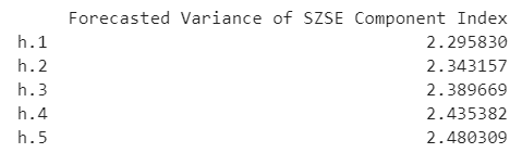
Figure 11: Forecast of Shenzhen Composite Index

Figure 11 showed the predicted results of SZSE Component Index with Garch model in five days.

3.3.2. Shanghai Composite Index forecasts

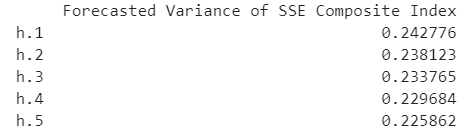
Figure 12: Forecast of Shanghai Composite Index

Figure 12 showed the predicted results of SSE Composite Index with Garch model in five days.

4. Discussion

This study employs logarithmic returns to smooth the data and facilitate a more detailed characterization of its attributes.

The adoption of the Generalized Auto-regressive Conditional Heteroskedasticity (GARCH) model in this paper provides an enhanced capacity to capture the long-term memory characteristics present in actual data, surpassing the capabilities of the Auto-regressive Conditional Heteroskedasticity (ARCH) model. The GARCH model is particularly adept at analyzing and predicting volatility, thereby offering significant guidance for investors' decision-making processes.

The implications of this model extend beyond mere numerical analysis and prediction.

The research data utilized in this study is sourced from a specialized stock platform, ensuring both authenticity and reliability of the data.

However, this study is confined to the GARCH model and lacks comparison with other potential models, limiting the ability to ascertain whether it is the most optimal and accurate model. Additionally, the analysis primarily focuses on the correlations between stock markets based on fluctuations in closing prices, neglecting other influential factors. The exclusive use of the GARCH model is recognized as a limitation [8].

Given the superficial understanding of the model and the lack of comprehensive analysis, future studies should aim for the following enhancements:

Future research could explore more complex parametric GARCH models, such as those incorporating Beta or Laplace distributions, which may yield more refined results [9].

Future investigations might also consider multiple aspects of stock performance, such as daily highs and lows, to examine potential correlations within the stock markets [10].

5. Conclusion

The examination of linear distribution charts for both the Shanghai Composite Index and the Shenzhen Component Index reveals that the distributions of returns exhibit multiple peaks and substantial fluctuations. This indicates a strong presence of abrupt changes and pronounced clustering of fluctuations.

Analysis of histograms and measures of skewness for the Shanghai Composite Index and the Shenzhen Component Index demonstrates that both indices are characterized by left-skewed distributions with kurtosis coefficients exceeding 3, indicative of leptokurtic distributions featuring sharp peaks and fat tails. Additionally, the positive mean values of these indices suggest that the economic landscape in China is currently in a state of growth. However, the relatively low standard deviation points to the immaturity of China’s stock market.

The derived formulas indicate that past fluctuations in the Shanghai Composite Index and the Shenzhen Component Index significantly influence current volatilities, contributing to a clustering effect of fluctuations. The returns of these indices display high persistence, underscored by strong speculative elements and heightened overall risks. Projections regarding the future trajectories of these indices have also been formulated based on these analyses.

References

[1]. Lin, Z. (2018). Modelling and forecasting the stock market volatility of SSE Composite Index using GARCH models. Future Generation Computer Systems, 79, 960-972.
[2]. Arashi, M., & Rounaghi, M. M. (2022). Analysis of market efficiency and fractal feature of NASDAQ stock exchange: Time series modeling and forecasting of stock index using ARMA-GARCH model. Future Business Journal, 8(1), 14.
[3]. Jiang, W. (2012). Using the GARCH model to analyse and predict the different stock markets. Uppsala University, 2-24.
[4]. Franses, P. H., & Van Dijk, D. (1996). Forecasting stock market volatility using (non‐linear) Garch models. Journal of forecasting, 15(3), 229-235.
[5]. Chong, C. W., Ahmad, M. I., & Abdullah, M. Y. (1999). Performance of GARCH models in forecasting stock market volatility. Journal of forecasting, 18(5), 333-343.
[6]. Lim, C. M., & Sek, S. K. (2013). Comparing the performances of GARCH-type models in capturing the stock market volatility in Malaysia. Procedia Economics and Finance, 5, 478-487.
[7]. Hajizadeh, E., Seifi, A., Zarandi, M. F., & Turksen, I. B. (2012). A hybrid modeling approach for forecasting the volatility of S&P 500 index return. Expert Systems with Applications, 39(1), 431-436.
[8]. Wang, Y., Xiang, Y., Lei, X., & Zhou, Y. (2022). Volatility analysis based on GARCH-type models: Evidence from the Chinese stock market. Economic research-Ekonomska istraživanja, 35(1), 2530-2554.
[9]. Franses, P. H., & Van Dijk, D. (1996). Forecasting stock market volatility using (non‐linear) Garch models. Journal of forecasting, 15(3), 229-235.
[10]. Bezerra, P. C. S., & Albuquerque, P. H. M. (2017). Volatility forecasting via SVR–GARCH with mixture of Gaussian kernels. Computational Management Science, 14, 179-196.
Cite this article
Luo,J. (2024). Utilizing the GARCH Model for Analysis and Prediction of Stock Market Trends. Advances in Economics, Management and Political Sciences,96,1-11.
Data availability
The datasets used and/or analyzed during the current study will be available from the authors upon reasonable request.
Disclaimer/Publisher's Note
The statements, opinions and data contained in all publications are solely those of the individual author(s) and contributor(s) and not of EWA Publishing and/or the editor(s). EWA Publishing and/or the editor(s) disclaim responsibility for any injury to people or property resulting from any ideas, methods, instructions or products referred to in the content.
About volume
Volume title: Proceedings of ICMRED 2024 Workshop: Identifying the Explanatory Variables of Public Debt and Its Importance on The Economy
© 2024 by the author(s). Licensee EWA Publishing, Oxford, UK. This article is an open access article distributed under the terms and
conditions of the Creative Commons Attribution (CC BY) license. Authors who
publish this series agree to the following terms:
1. Authors retain copyright and grant the series right of first publication with the work simultaneously licensed under a Creative Commons
Attribution License that allows others to share the work with an acknowledgment of the work's authorship and initial publication in this
series.
2. Authors are able to enter into separate, additional contractual arrangements for the non-exclusive distribution of the series's published
version of the work (e.g., post it to an institutional repository or publish it in a book), with an acknowledgment of its initial
publication in this series.
3. Authors are permitted and encouraged to post their work online (e.g., in institutional repositories or on their website) prior to and
during the submission process, as it can lead to productive exchanges, as well as earlier and greater citation of published work (See
Open access policy for details).