1. Introduction

1.1. Idea

We determine industry leading stocks based on LLR, and then use correlation analysis to take the lagging stocks with strong correlation with the leading stocks as our stock pool. Widespread intercorporate ownership might also cause firm fundamentals to move together [1], as this implicitly causes some firms’ performance to depend on that of other firms control for size effects in examining the cross-autocorrelation patterns between high volume and low volume stocks. When the leading stock rises by the limit, buy the corresponding lagging stock, and according to the variance and closing price of the leading stock's capital flow, the large fluctuation of the leading stock price is used as a short signal. If the market is efficient, mispricing will be quickly corrected, stocks with abnormal performance will not maintain the performance subsequently [2]. We monitor every day and find that when the leading stocks no longer rise by the daily limit, we believe that leading stocks are ineffective, so we sell the stocks we were long on at this time. When the volatility of leading stocks returns to normal, we will return the stocks we shorted before.

1.2. Highlight

The top 10% of stocks were selected based on the ranking by the LLR index of stocks in several industries as the leading stocks, and the lagging stocks were determined by computing the correlation coefficient between other stocks in the same industry and leading stocks to build a portfolio. For data accuracy, the study monitors the daily LLR records. We buy the corresponding trend of lagging stocks when the leading stocks appear limit signals. In addition, by calculating the variance of the leading stock, we believe that if the standard variance mean ratio is greater than or equal to 0.02, the stock will have a large fluctuation, and we will use this as a signal to short the corresponding lagging stock. The law is that once the daily purchase monitoring, the leading stocks in the industry will no longer rise by the limit, which means the failure of the leading stocks, once the leading stocks fail, we will sell the corresponding industry to follow the trend of lagging stocks; Once the standard variance mean ratio of the leading stock shorted is less than 0.02, the corresponding lagging stock that was shorted before will be closed.

2. Specification

2.1. Analysis

2.1.1. Qualitative analysis

China's stock market is not mature compared to developed countries; there is a huge information asymmetry. For instance, the market information disclosure system is incomplete due to improper data records and collection, which leads to a serious information gap in the stock market. Therefore, it is difficult for investors to get a completely true operating situation of the listed company's financial statements and their performance since falsification of the financial statement is common. Also, there are many individual investors in China's stock market, and the investment expertise of individual investors has contributed mainly to falsifying financial records due to the phenomenon of following the herd, and the "herding effect" is significant.

2.1.2. Quantitative analysis

First we use lead-lag ratio (LLR) to study the relationship between the two assets after the lead, based on the LLR model we can determined the leading stocks in the market. then we use R² and accuracy as dependent variables to detect the real existence of the leading driving effect of leading stocks, which has a predictive effect on other lagging stocks in the sector, if the value of R² is big enough (over 0.6), then we reckon the two stocks have a strong correlation.

We use the basic mathematical statistics theory to give a quantitative index to measure the stock price volatility -- standard variance mean ratio, and use this index to divide the volatility into normal volatility and abnormal volatility. And for the standard deviation mean ratio, we obtained A reference value of 0.02 based on the Shenzhen Stock Exchange A-share index.

2.2. Data--Universe & Datasets & Data Sources & Data Range

The study will use secondary sources and adopts a quantitative research method. The research design used is explanatory research using descriptive and inferential statistics to analyze the data. The data is selected randomly for the opening and closing prices from January 2, 2018, to July 17, 2023. The data is inserted in Excel, cleaned through format unification, data standardization, consistency check, and coded before analysis in the Stata software. To get the return of each stock, we subtract the closing price of the current day from the previous day's closing price and divide the previous day's closing price to get the return of each stock. In addition, since the market yield is difficult to obtain, we believe that dividends have been reflected in the fluctuations of the stock index. The market index is used as a customary substitute for the market yield. The research will use the CSI 300 index as our daily market yield for accuracy. Also, to obtain the variance of the return rate of each stock and the variance of the market return rate, we prepare the data for the subsequent calculation of the correlation coefficient between the leading stock and other stocks in the trading industry. In addition, we also use data on the flow of funds. Moreover, for the standard variance mean ratio, we obtained A reference value of 0.02 based on the Shenzhen Stock Exchange A-share index.

For the back test data, we selected the data from January 2, 2018, to January 2, 2021, as in-sample data and from January 2, 2021, to July 17, 2023, as out-sample data [3].

2.3. Methodology

2.3.1. Signal Generation

A signal to long:

Different trading sectors in China have different daily stock limits. Therefore, once the leading stocks in a given industry appear to have reached their daily limit phenomenon, it will be good news for the industry since they will play a leading role in the lagging stocks [4]. Therefore, the lagging follower stocks will have a trend to approach the leading stocks in the future. Hence, the daily limits of leading stocks will be used as the signal.

For the main board, the equation can be expressed as follows;

\( \frac{{P_{c(n)}}}{{P_{o(n)}}}≥0.1 \)

For the science and technology board, the equation can be expressed as follows;

\( \frac{{P_{c(n)}}}{{P_{o(n)}}}≥0.2 \)

When the growth rate of the leading stock reaches the limit of its module, we will use it as a buy signal and buy the portfolio of the corresponding industry of the leading stock.

A signal to short:

By calculating the standard variance mean ratio, the price fluctuation of leading stocks can be obtained.

\( \bar{{X_{n}}}=\frac{1}{5}\sum _{i=n-2}^{n+2}{X_{i}} \)

\( {S_{n}}=\sqrt[]{\frac{1}{4}\sum _{i=n-2}^{n+2}{({X_{i}}-\bar{{X_{n}}})^{2}}} \)

\( {W_{n}}=\frac{{S_{n}}}{\bar{{X_{n}}}} \)

When the standard variance mean ratio is greater than or equal to the reference value of W₀=0.02, we believe that the price of leading stocks is relatively volatile, and we use this as a signal to short lagging stocks with strong correlation with leading stocks.

2.3.2. Portfolio Construction-Sizing & Timing of trading & Input-output Ratio

2.3.2.1. Sizing

(1) The first step is to find the leading stocks in the industry.

For two stocks, X and Y (assuming X is the leader and Y is the laggard),

\( \frac{\sum _{i=1}^{p}{(ρ(i))^{2}}}{\sum _{i=1}^{p}{(ρ(-i))^{2}}} \gt 1 \)

Huth and Abergel defined the left side of the inequality of the formula (3-1) as the Lead lag ratio (LLR) [5].

\( ρ(i)=Corr(r_{t}^{Y},r_{t-i}^{X}) \)

\( LLR=\frac{\sum _{i=1}^{p}{(ρ(i))^{2}}}{\sum _{i=1}^{p}{(ρ(-i))^{2}}} \)

( \( \lbrace r_{t}^{X}\rbrace \) : stock X's return series, \( \lbrace r_{t}^{Y}\rbrace \) : stock Y's return series)

When LLR>1, I can judge stock X as the leading stock and stock Y as the lagging follower stock.

Then extend this property to multiple stocks, expand to an entire industry, \( win\_num \) and \( \bar{LLR} \) indicators to sort the stocks in the sector, select the top 10% of the stocks in the sector as leading stocks;

\( win\_num \) :

If there are N stocks in A sector and LLR is calculated by combining this stock with other stocks in pairs to obtain N-1 LLR, then \( win\_num \) is defined as the number of LLR>1, the number of times a stock has performed better than another stock.

\( \bar{LLR} \) :

So far we have learned that according to LLR & gt; 1 can determine that X is more leading than Y, but it is worth noting that the greater the LLR is greater than 1, the stronger X is leading. Therefore, set \( \bar{LLR} \) to calculate the average LLR of each stock to make a more reasonable ranking of stocks in the sector.

\( \bar{LLR}=MEAN(LLR) \)

After completing the LLR index ranking of stocks in various industries, we select the top 10% stocks as leading stocks.

(2) In the second step, the study will determine the lagging stocks in our portfolio. Once the leading stocks are identified through the relationship, we select which stocks in the same industry have a leading role, that is, to select lagging stocks. According to statistician Carl Pearson, the correlation coefficient can be used to measure the degree of linear correlation between variables. Therefore, we evaluate the correlation coefficient between other stocks in the same industry and leading stocks as follows [6];

\( {R^{2}}=\frac{{β^{2}}α_{m}^{2}}{{β^{2}}σ_{m}^{2}+σ_{ε}^{2}} \)

( \( σ_{m}^{2} \) : the variance of market returns, \( σ_{ε}^{2} \) : the variance of individual stock returns, \( β \) : The leading stocks are the explanatory variables and individual stocks are the regression coefficients of the explained variables)

Next, we choose lagged stocks greater than 0.6 to construct our investment portfolio. According to the Shanghai Stock Exchange data, it divides the stocks of listed companies into 91 sub-sectors (appendix.). For this purpose, we will find the leading and lagging stocks in each industry and construct the portfolio of each module to form a large portfolio pool.

2.3.2.2. Timing of trading

After completing the portfolio purchase, we monitor LLR daily to check whether there is still a leading effect of leading stocks on lagging stocks on that day.

The trading time for going long is when the leading stocks rise by the limit of the trailing stocks corresponding to our going long; If the leading stock still reach its price limit, which means there is still a leading effect, we continue to hold positions; If the leading stock fails, we sell the portfolio of the industry corresponding to the failed leading stock [7].

Short trading time is when the price of the leading stock is very volatile, that is, its standard variance mean ratio is greater than or equal to 0.02. When the standard mean variance of the leading stock is less than 0.02, we will pay back all the stocks that were previously shorted.

2.3.3. Allocation of stock investment funds

Assuming that our total investment amount is $1 million.

First, we calculate the variance of the capital flow of leading stocks in each industry, and set the variance of the industry with long position as positive, and the variance of the industry with short position as negative.

The resulting variance is then multiplied by a fixed percentage to get the amount of investment we allocate to different industries.

\( {G_{i}}=Var(fund flow)*porpotion \)

\( porpotion=\lbrace 0,\frac{1}{n},\frac{2}{n}……\frac{n-1}{n},1\rbrace \)

\( \bar{G}=\frac{{G_{i}}}{\sum _{i=1}^{5}{G_{i}}} \)

\( normalize {G_{i}}={G_{i}}-\bar{G} \)

Finally, in various industries, we allocate funds for each stock according to the correlation coefficient between the trailing stocks and the leading stocks selected by us. The stronger the correlation is, the more funds we will invest.

\( {ω_{i}}=C\frac{{R_{i}}}{\sum _{i=1}^{p}{R_{i}}} \)

( \( {ω_{i}} \) : The amount of money invested in each stock, C: Total investment amount, \( {R_{i}}: \) The regression coefficient of each stock to the leading stock)

2.3.4. Trade Execution

2.3.4.1. Fee cost

In our strategy, we based on the average fee cost in China market and set the fee cost equal 0.06% of the total funds, which are taken as a commission according to the exchange regulations.

2.3.4.2. Opportunity Cost

Because we are monitoring the leading stocks to determine whether to buy or sell lagging stocks, we lose the opportunity to buy leading stocks.

3. Results-- (In-sample performance)

3.1. P&L Graph (Figure 1) & Summary Statistic

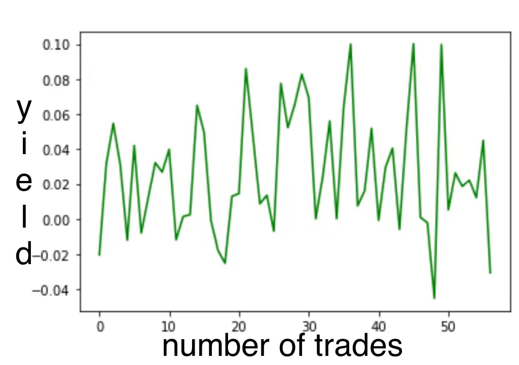
Figure 1: P&L Graph

3.2. Abnormal Analysis

In this trade, we saw an instant drop in the yield on days 45 to 48. And before that, good returns were guaranteed for some time. This phenomenon shows that the leading stock driving effect needs to be detected in time. Otherwise, in the short term, because of the purchase of many stocks, the decline of the sector will lead to a significant reduction in earnings.

4. Refinements

(1) We recommend that investors establish appropriate stop-loss points when using the strategy. This strategy has not yet considered the stop-loss point. Still, it can not be ignored that unexpected situations in the market, such as false signals or excessive confidence, make the leading stock's driving effect on other stocks in the same industry ineffective and may also bring unreasonable plummeting. Therefore, to further avoid risks, it is recommended that investors use this strategy based on setting a reasonable stop-loss point.

(2) We recommend that investors consider the LLR distribution where possible. When sorting LLR indicators in this strategy, \( \bar{LLR} \) is also used as one of the indicators. Although it can make up for some defects of the indicators and reduce the possibility of stocks with the same ranking to a certain extent, since \( \bar{LLR} \) is the average value is calculated? If the LLR distribution is relatively discrete and there are more extreme values, \( \bar{LLR} \) may not be a good ranking indicator. Because it is largely affected by extreme values, a more detailed judgment can be made by considering the LLR distribution to make the strategy more reasonable.

5. Conclusion

5.1. Out-of-sample performance

The average daily yield is 0.0499%.

5.1.1. P&L Graph & Summary Statistic

Going long (Figure 2):

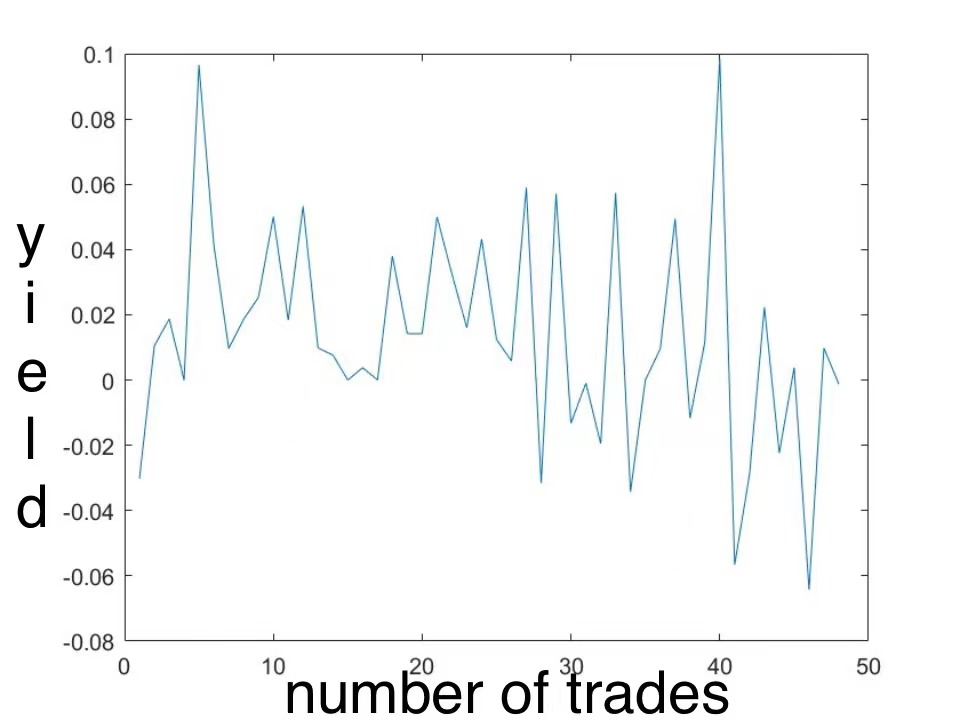
Figure 2: P&L Graph (Going long)

Short-selling (Figure 3):

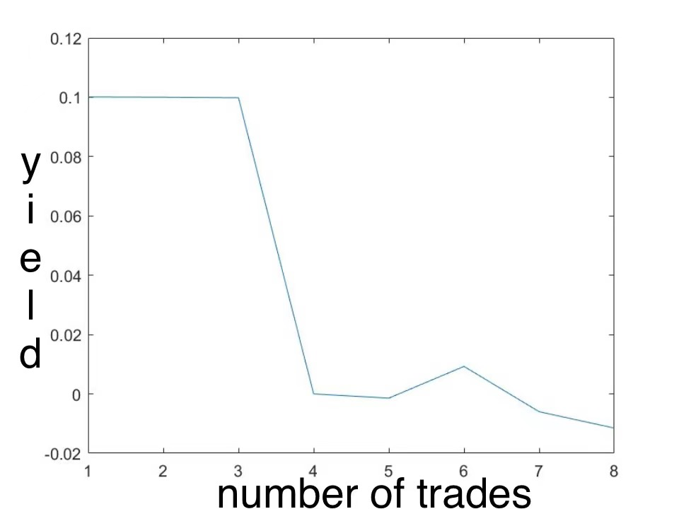
Figure 3: P&L Graph (Short-selling)

5.1.2. Abnormal Analysis

The test was taken from data starting in 2021, which was later affected by the epidemic, resulting in the Chinese stock market being heavily affected and volatile. Therefore, this strategy is greatly affected by macroeconomic conditions, and all in risk is greater.

5.2. Trading Recommendation

Based on our investment strategy, we recommend that investors who adopt this scheme consider as much as possible the LLR of leading stocks, and do as much testing as possible. For China's A-share market and B-share market, the daily limit is a rare trend. And for our strategy, once the daily limit signal disappears, we must sell all of them. Therefore, real-time detection of LLR data is a very important point. And based on the reason of poor information, the detection of LLR has a delay. Therefore, frequent detection of LLR can help us reduce risks and avoid excessive losses.

The second is to ensure the correctness of real-time data. For the Pearson correlation function, once it is lower than 0.6, it belongs to medium correlation and below. So once it is below 0.6, our strategy will lose its meaning and fail to work successfully.