


1. Introduction
China's Margin Trading and Short Selling Unwinding Pilot Program in 2010 marked a turning point in the Chinese stock market. This initiative led to the exploration of pair trading strategies for enhanced investment. Pair trading, pioneered by Nunzio Tartaglia in the 1980s, gained popularity among investors and traders. It involves identifying two stocks with long-term price equilibrium, taking both long and short positions when prices deviate, and profiting when the spread reverts. The process entails selecting asset pairs and identifying opportunities. Cointegration theory is favored for pair selection due to its proven profitability. A systematic analysis of a diverse pool of stocks is crucial. It's essential to differentiate between correlation and cointegration. After identifying cointegrated stocks, trading signal tests and strategies are proposed. This approach ensures profitability while minimizing potential losses in volatile scenarios [1].
2. Literature review
2.1. Introduction to pairs trading
Elliott defines pairs trading as a strategy exploiting temporarily imbalanced financial markets, involving a long position in one security and a short position in another at a predetermined ratio [2]. This approach capitalizes on market deviations from equilibrium, presenting profit opportunities. Traders create a self-financing portfolio by taking long positions in undervalued assets and short positions in overvalued ones, closing positions upon convergence for profit. Rad categorizes Pairs Trading Strategy (PTS) as a form of statistical arbitrage within finance. This approach employs statistical models or methods to exploit potential pricing discrepancies in assets while maintaining market neutrality [3]. Furthermore, the concept of PTS extends to analyzing equilibrium relationships in financial markets and constructing portfolios of securities, encompassing both short and long positions [4].
2.2. The Correlation Method
The correlation method involves selecting pairs of stocks based on their correlations between returns. While Chen et al. [5] demonstrated significant returns over an extended period, it's important to note their study didn't account for transaction costs, potentially overestimating returns.
2.3. The Cointegration Method
The cointegration method employs time series analysis to determine if a linear combination of two non-stationary time series can yield a stable, predictable trend. Engle and Granger introduced a "two-step cointegration test" to identify these trends, a method further examined by Doldado et al. [6]. They emphasized how this test formalizes the notion of variables sharing an equilibrium relationship among time series. Traders initiate a market-neutral arbitrage portfolio when the spread exceeds the predetermined number of standard deviations from the historical mean.
2.4. The distance method
Gatev et al. [7] introduced the Distance Method (DM) as a supposedly profitable pairs trading strategy. However, Krauss [8] critiqued it, arguing that an 'ideal pair' with a spread of zero would yield no profits, as the method tends to select pairs with limited profit potential. Further analysis by Do and Faff [9] revealed a declining profitability trend, attributed to a reduction in arbitrage opportunities. They concluded that the DM strategy became significantly unprofitable after 2002, particularly when considering trading costs [10].
2.5. The Copula Method
The copula method, employing probabilistic modeling of stock price distributions, shows promise in academic circles due to its strong theoretical basis and positive outcomes in limited applications. However, Rad, Low, and Faff caution that in broader contexts, it falls significantly behind the cointegration and distance methods [3]. Given the inconsistent performance of the distance and copula methods, this study opted not to implement them, using them instead as benchmarks to evaluate the pairs selection algorithms in this study.
3. Methods
3.1. Overview
This study employs data from 73 Chinese technology stocks and 6 metal futures spanning from 8/3/2017 to 8/3/2023 for pair trading. The process involves two stages: pair formation and simulated trading strategies. In the pair formation stage, pairs are identified using correlation and cointegration methods. Correlation maximization and rigorous statistical tests for cointegration are employed. The top five pairs with the lowest cointegration test values are selected. Moving to the second stage, trades are executed for the identified pairs. Determining the timing for positions is crucial. This is guided by the generated ratio time series. A predictor variable, YY, is created. Positive values indicate a "buy" recommendation, while negative values signify a "sell" recommendation. The predictive model structure is outlined as follows: \(Yt=sign(Ratiot+1-Ratiot)\) The advantage of pair trading signals lies in the fact that the determination of the absolute price direction is not required; instead, the focus of this study is solely on discerning the price movement: whether it is trending upwards or downwards.
3.2. Data
In order to engage in pairs trading effectively, it is essential to limit the selection of securities to a specific industry. This ensures that there exists a meaningful economic correlation between the chosen pairs, facilitating a more straightforward evaluation of trading performance. After considering data comprehensiveness and diversity across various sectors, stocks and metal futures associated with the technology sector were identified as the subjects of this study. The selected technology sector stocks encompass ‘000050.SZ’ (Tianma Microelectronics Co., Ltd.), ‘000670.SZ’ (Infotmic Co., Ltd.), ‘001339.S’Z (JWIPC Technology Co., Ltd.), ‘688385.SS’ (Shanghai Fudan Microelectronics Group Company Limited), ‘688357.SS’ (Luoyang Jianlong Micro-nano New Material Co., Ltd ), ‘688699.SS’ (Shenzhen Sunmoon Microelectronics Co.Ltd), ‘688582.SS’ (Anhui XDLK Microsystem Corporation Limited), ‘688728. SS’ (GalaxyCore Inc.) and others. Additionally, the selected metal futures comprise ‘SI=F’ (Silver), ‘GC=F’ (Gold), ‘HG=F’ (Copper), ‘ALI=F’ (Aluminum), ‘PA=’F (Palladium) and ‘PL=F’ (Platinum). Initially, this study encompassed all trading dates spanning from 8/3/2017 to 8/3/2023, constituting a continuous six-year period. Certain securities failed to meet the established criteria, possessing less than six years' worth of data. They were excluded based on their data availability.
3.3. The Correlation Method
The correlation statistic is employed for the preliminary selection of potential stocks to further refine the trading pairs. This is due to its ability to pinpoint stocks that are highly correlated. The following section will delve into the formal mathematical foundation of correlation. Given two stocks, denoted as X and Y, let \(P^X\) and \(P^Y\) represent their respective prices. The Pearson Correlation Coefficient ( \(\rho\) ) is employed to quantify the correlation between stocks X and Y, as shown in equation 1.
where \( \mathrm{T} \) is the observation over the investigated period,and \( \overline{\boldsymbol{P}}^{\boldsymbol{X}}\) and \(\overline{\boldsymbol{P}}^{\boldsymbol{Y}} \) denote the mean prices of stocks \( \mathrm{X} \) and \( \mathrm{Y} \) , respectively, which are given by \(\bar{P}^{X}=\frac{1}{T} \sum_{t=1}^{T} P_{t}^{X} \text ,\bar{P}^{Y}=\frac{1}{T} \sum_{t=1}^{T} P_{t}^{Y}\) The Pearson Correlation Coefficient ( \(\rho{XY}\) ) quantifies the strength of the relationship between two stocks, X and Y, and ranges from -1 to 1. A higher positive value of ( \(\rho{XY}\) ) signifies a stronger positive correlation between stocks X and Y. A threshold of ( \(\rho{XY}\) ) = \(\pm\) 0.50 is established to select stock pairs. By using correlation coefficients as a filter, the correlation matrix of the chosen stocks at time t is obtained. Correlation coefficients serve as a criterion for prioritizing and selecting stock pairs. The pairs with the highest correlation coefficients are then chosen. However, relying exclusively on the correlation method for pair trading has its drawbacks since the prices of paired stocks can become volatile overtime. It's important to note that a high correlation coefficient doesn't guarantee a mean reversion between the prices of the two stock pairs. This is primarily due to the fact that the correlation method is sensitive to even minor temporal deviations (Harris, 1995; Lin, McCrae, \textbackslash{}\& Gulati, 2006), especially within the realm of high-frequency dynamic pair trading. To overcome these issues, the cointegration approach was adopted as the second step of the analysis.
3.4. The Cointegration Method
Cointegration, a fundamental concept in time series analysis, denotes a sustained synchronicity between two variables. Central to cointegration is the concept of stationarity, the property of a time series where its statistical characteristics remain unchanged over time, signifying a consistent relationship between past and future values. The cointegration method establishes a linear relationship between two nonstationary time series, determining if the result is stationary. The well-regarded Engle-Granger Two-step method is a prominent approach. It involves regressing one time series variable against the other to estimate coefficients, followed by an analysis of the residuals for stationarity. This is achieved by using the Augmented Dickey-Fuller (ADF) test for existence of unit root. If the residual series has a unit root, it is influenced by its past values and thus non-stationary. On the other hand, the Johansen Cointegration Test accommodates complex scenarios with multiple variables but is not the primary choice for the specific focus on two variables. In the analysis, the Engle-Granger method was applied to ascertain cointegration among microelectronic component stocks in the Chinese market and selected metal futures in the esteemed New York Mercantile Exchange (NYMEX). After filtering out stationary assets, this method yielded valuable insights into the enduring relationships within the chosen portfolio.
3.5. Trading Strategy
After assessing covariance among currency pairs, the next step involves generating trading signals. This includes introducing a "Ratio" variable to record daily ratio values between predicted and target closing values. The ratio is standardized by subtracting the mean and dividing by the standard deviation, setting upper and lower Z-score bounds at 1 and -1 respectively. The dataset includes six columns: (i) Date; (ii) Asset 1 (closing value of the first stock); (iii) Asset 2 (closing value of the second stock); (iv) Z-score (normalized ratio value); (v) Upper Limit (all entries assigned 1); and (vi) Lower Limit (all entries assigned -1). Using the Z-score, trading signals for Asset 1 are generated. If the Z-score exceeds the upper limit, a short strategy is implemented; otherwise, a long strategy is employed. A "Signal 1" column is added to the Signal Data Frame, with -1 for short and 1 for long. A "Signal 2" column is added for Asset 2, with opposite signs to Signal 1. To identify undervalued opportunities, two columns are added to the signaling data frame. "Position 1" for Asset 1 is computed based on first-order differences in "Signals 1". Similarly, "Position 2" for Asset 2 is determined by differences in "Signals 2". A value of 0 in "Position 1" indicates no change, 1 signifies a transition from 0 to 1, and -1 denotes a change from 1 to 0. Entries in "Positions 2" follow a similar logic. Finally, portfolio returns are calculated. For each day in the test period, the sum of holding value and cash amount of both stocks is recorded as "total portfolio value". On August 4, 2023, this value is used to determine profit or loss, and subsequently, the portfolio's return is computed.
4. Result
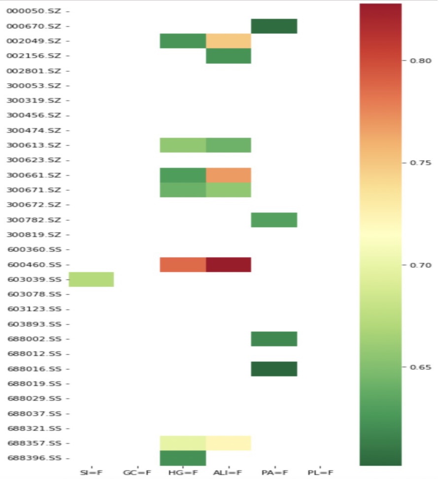
This section presents detailed performance results for a portfolio of technology sector stocks and metals futures pair-trading. Yahoo Finance and Python 3.9.7 with relevant libraries are used for data extraction for pair-trading. As shown in Figure 1, the top five pairs of highly correlation were selected. The five pairs are (i) ('600460.SS' and 'ALI=F'), (ii) ('600460.SS' and 'HG=F), (iii) ('300661.SZ' and 'ALI=F'), (iv) ('002049.SZ' and 'ALI=F) and (v) ('688357.SS' and 'ALI=F').
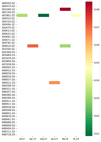
However, since highly correlated pairs do not necessarily exhibit the degree of cointegration, the next step involves employing the cointegration method to identify the pairs with which should be engaged in pair trading. As shown in Figure 2, using the cointegration method, the five pairs are (i) (HG=F and 002801.SZ, 0.008427659652707312), (ii) (PA=F and 300819.SZ, 0.03037450319347318), (iii) (SI=F and 002801.SZ, 0.03252089745046688), (iv) (PL=F and 002801.SZ,0.045964704477125376) and (v) (ALI=F and 688211.SS, 0.06529101754510638)
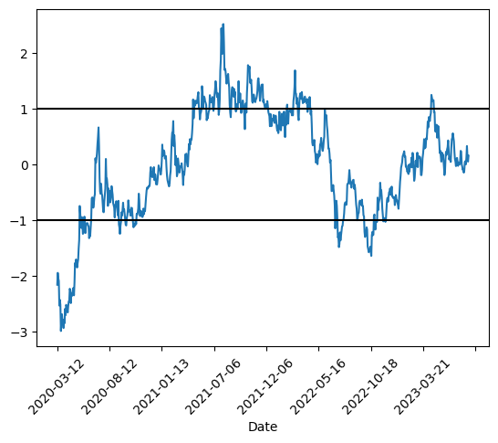
At this point, visualization of the spread between the two time series was done. This is achieved by employing linear regression to establish a linear combination of coefficients derived from the two securities. Alternatively, opting to analyze the ratio between the two time series is also possible. Figure 3 depicts a plot of the z-values of the ratio series and their upper and lower bounds. By adding two extra lines below the Z-scores of 1 and -1, is is clearly observed that in most cases, any significant deviations from the mean will eventually converge. This aligns with the trading strategy that this study aims for.
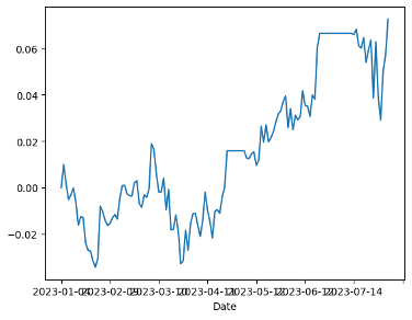
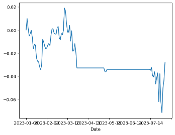
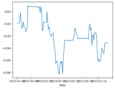
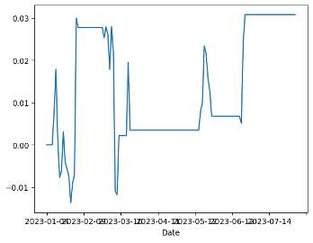
It is crucial to identify the pertinent features that influence the direction of the ratio movements. Considering the consistent reversion of ratios back to the mean, metrics associated with moving averages and those related to the mean could potentially hold significance. It is noteworthy that a time series comprising 252 data points was utilized, aligning with the number of trading days in a year. These parameters were used: 30 day Moving Average of Ratio, 5 day Moving Average of Ratio, 30 day Standard Deviation, z-score, (5d MA - 30d MA)/ 30d SD Figure 4a displays PL=F and 002801.SZ without using a stop-loss strategy. In Figure 4b, the impact of setting the stop-loss limit as the z-value plus tolerance is observed. After implementing the z-value plus tolerance stop-loss limit, the results indicate a reduction in volatility. While the return without a stop-loss stands at approximately 80 percent, a decreasing in return implementing the stop-loss limit is observed.
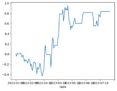 (a) PL=F and 002801.SZ without setting a stop loss
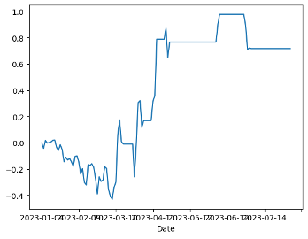 (b) PL=F and 002801.SZ setting a stop loss
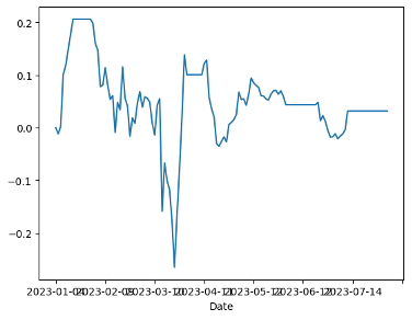
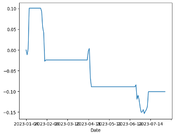
Figure 5a displays HG=F and 002801.SZ without a stop-loss strategy. In Figure 5b, the impact of setting the stop-loss limit as the z-value plus tolerance is shown. After implementing the z-value plus tolerance stop-loss limit, the results indicate an increase in earnings, and the holding period is as of May 2023. This strategy did not yield any returns before, but now it has generated an income of about 3 percent.
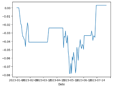 (a) HG=F and 002801.SZ without setting a stop loss
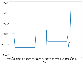 (b) HG=F and 002801.SZ setting a stop loss
Figure 6a displays PA=F and 300819.SZ without a stop-loss strategy. In Figure 6b, the impact of setting the stop-loss limit as the z-value plus tolerance is shown. After implementing the z-value plus tolerance stop-loss limit, the results indicate a negative correlation. There is an adverse effect attributed to the stop-loss limit, especially when positions exceed the defined tolerance.
 (a) PA=F and 300819.SZ without setting a stop loss
 (b) PA=F and 300819.SZ setting a stop loss
Figure 7a displays ALI=F and 688211.SS without a stop-loss strategy. In Figure 7b, we can observe the impact of setting the stop-loss limit as the z-value plus tolerance. After implementing the z-value plus tolerance stop-loss limit, it becomes evident that the stop-loss order is consistently triggered.
 (a) ALI=F and 688211.SS without setting a stop loss
 (b) ALI=F and 688211.SS setting a stop loss
Figure 8a displays SI=F and 002801.SZ without a stop-loss strategy. In Figure 8b, the impact of setting the stop-loss limit as the z-value plus tolerance is shown. The results indicate a positive impact. The tolerances are set so small that the stop-loss orders are frequently triggered. After implementing the stop-loss limit, the revenue was approximately 3 percent.
 (a) SI=F and 002801.SZ without setting a stop loss
 (b) SI=F and 002801.SZ setting a stop loss
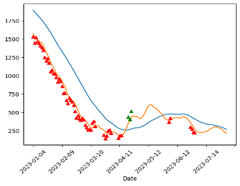
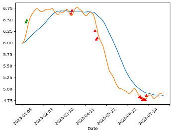
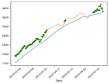
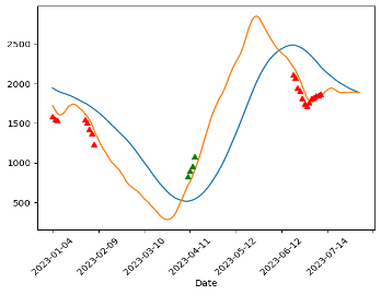
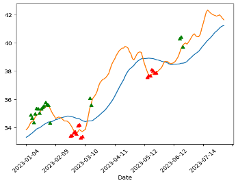
Trade signals are prompts to either buy or sell securities or other assets, and these prompts are generated through analytical processes. This analysis can be derived from technical indicators or mathematical algorithms that rely on market behaviors. It may also incorporate other market factors like economic indicators for a comprehensive assessment. The pair-trading signal points are plotted from Figure 9 to Figure 13. The red markers are buys and the green markers are sells.
5. Conclusion
Using rigorous statistical analysis, the viability of pairs trading strategies in today's financial markets is confirmed. Testing two distinct methodologies using recent data reveals profitability through both correlation and cointegration approaches. Further algorithm refinement, including intraday data integration and stop-loss mechanism optimization, is anticipated to enhance returns. Despite potential improvements, the cointegration method proves robust in generating substantial returns, even in challenging economic conditions. This study underscores the enduring relevance of statistical arbitrage, supported by the pairs trading results. It is crucial to closely examine the foundational relationships among arbitrage pairs, particularly in a dynamic corporate landscape where shifts can occur rapidly. The stock selection strategy in this study focuses on companies closely linked to selected commodity futures in their production processes. With more extensive data, uncovering assets with less apparent correlations could be expected, further enhancing profitability. While the test results received positive feedback, there are limitations. With more time, expanding the study by adding statistical arbitrage methods and a broader dataset would be fruitful. Cumulative returns have room for optimization, potentially avoiding losses. Daily trading may not capture all market information effectively. Applicability might vary across sectors and industries. Cointegration can occur across different industries and countries. Refining grid searches and using advanced optimization methods can enhance results. Further research is needed, particularly for methods requiring explicit functions. Improving trading simulations can increase robustness, and threading integration can enhance program efficiency.
References
[1]. G.J. Miao, High frequency and dynamic pairs trading based on statistical arbitrage using a two-stage correlation and cointegration approach, Int. J. Econ. Finance 6 (2014) 96–110.
[2]. Quantitative Elliott, Robert J., John Van Der Hoek, and William P. Mal- colm. ”Pairs trading.”
[3]. Quantitative Finance, 16(10):1541–1558, 2016. H. Rad, R. K. Low, and R. Faff. The profitability of pairs trading strategies: Distance, cointegration and copula methods.
[4]. Finance 5.3 (2005): 271-276. Nicholas, J.G., Market Neutral Investing— Long/Short Hedge Fund Strategies, 2000 (Bloomberg Professional Library, Bloomberg Press: Princeton, NJ, USA).
[5]. Management Science, 65(1):370–389, 2019. H. J. Chen, S. J. Chen, Z. Chen, and F. Li. Empirical investigation of an equity pairs trading strategy.
[6]. Journal of Economic Surveys, 4(3):249–273, 1990. J. J. Dolado, T. Jenkin- son, and S. Sosvilla-Rivero. Cointegration and unit roots.
[7]. Review of Financial Studies 19 (3), 797–827. Gatev, E., Goetzmann, W. N., Rouwenhorst, K. G., 2006. Pairs trading: Performance of a relative value arbitrage rule
[8]. Journal of Economic Surveys, 31(2):513–545, 2016. C. Krauss. Statistical arbitrage pairs trad-ing strategies: Review and outlook.
[9]. Financial Analysts Journal 66 (4),83–95. Do, B., Faff, R., 2010. Does simple pairs trading still work?
[10]. Journal of Financial Research 35 (2), 261–287. Do, B., Faff, R., 2012. Are pairs trading profits robust to trading costs?
Cite this article
Liu,Y.;Gao,M.;Guo,Y.;Qiao,Y. (2024). Designing Efficient Pair-Trading Strategies for the Technology Stock Market. Advances in Economics, Management and Political Sciences,106,359-369.
Data availability
The datasets used and/or analyzed during the current study will be available from the authors upon reasonable request.
Disclaimer/Publisher's Note
The statements, opinions and data contained in all publications are solely those of the individual author(s) and contributor(s) and not of EWA Publishing and/or the editor(s). EWA Publishing and/or the editor(s) disclaim responsibility for any injury to people or property resulting from any ideas, methods, instructions or products referred to in the content.
About volume
Volume title: Proceedings of the 3rd International Conference on Business and Policy Studies
© 2024 by the author(s). Licensee EWA Publishing, Oxford, UK. This article is an open access article distributed under the terms and
conditions of the Creative Commons Attribution (CC BY) license. Authors who
publish this series agree to the following terms:
1. Authors retain copyright and grant the series right of first publication with the work simultaneously licensed under a Creative Commons
Attribution License that allows others to share the work with an acknowledgment of the work's authorship and initial publication in this
series.
2. Authors are able to enter into separate, additional contractual arrangements for the non-exclusive distribution of the series's published
version of the work (e.g., post it to an institutional repository or publish it in a book), with an acknowledgment of its initial
publication in this series.
3. Authors are permitted and encouraged to post their work online (e.g., in institutional repositories or on their website) prior to and
during the submission process, as it can lead to productive exchanges, as well as earlier and greater citation of published work (See
Open access policy for details).
References
[1]. G.J. Miao, High frequency and dynamic pairs trading based on statistical arbitrage using a two-stage correlation and cointegration approach, Int. J. Econ. Finance 6 (2014) 96–110.
[2]. Quantitative Elliott, Robert J., John Van Der Hoek, and William P. Mal- colm. ”Pairs trading.”
[3]. Quantitative Finance, 16(10):1541–1558, 2016. H. Rad, R. K. Low, and R. Faff. The profitability of pairs trading strategies: Distance, cointegration and copula methods.
[4]. Finance 5.3 (2005): 271-276. Nicholas, J.G., Market Neutral Investing— Long/Short Hedge Fund Strategies, 2000 (Bloomberg Professional Library, Bloomberg Press: Princeton, NJ, USA).
[5]. Management Science, 65(1):370–389, 2019. H. J. Chen, S. J. Chen, Z. Chen, and F. Li. Empirical investigation of an equity pairs trading strategy.
[6]. Journal of Economic Surveys, 4(3):249–273, 1990. J. J. Dolado, T. Jenkin- son, and S. Sosvilla-Rivero. Cointegration and unit roots.
[7]. Review of Financial Studies 19 (3), 797–827. Gatev, E., Goetzmann, W. N., Rouwenhorst, K. G., 2006. Pairs trading: Performance of a relative value arbitrage rule
[8]. Journal of Economic Surveys, 31(2):513–545, 2016. C. Krauss. Statistical arbitrage pairs trad-ing strategies: Review and outlook.
[9]. Financial Analysts Journal 66 (4),83–95. Do, B., Faff, R., 2010. Does simple pairs trading still work?
[10]. Journal of Financial Research 35 (2), 261–287. Do, B., Faff, R., 2012. Are pairs trading profits robust to trading costs?