1. Introduction

Gold is one of the world's most significant financial assets. In the contemporary gold market, the physical trading volume represents less than 3% of the total trading volume. This indicates that the majority of the market trading body is comprised of financial derivatives. The price fluctuations of gold exert a noteworthy influence on the economy, financial markets, and investors' decisions. In spite of the 2008 global financial crisis, the price of gold exhibited a notable increase, diverging from the trajectory of other financial products [1, 2]. This phenomenon suggests that in a context of heightened uncertainty, the allocation of gold as a hedge asset may be a prudent strategy. Therefore, it is very important to study the future direction of the gold price.

In the field of finance, the ability to forecast the price of financial products is of paramount importance. Many practitioners are developing models, including linear regression models, dynamic models, one-factor and multi-factor approaches. However, despite these efforts, the models still face valid criticisms [3]. The field of finance is characterized by a high degree of complexity and nonlinearity, with a multitude of other factors playing a role in estimating the relationship between potential predictors and expected returns. The study of gold price and trend forecasting and the factors influencing it has been conducted for decades, during which numerous methods have been proposed. For instance, the topic of predicting the price of gold has been approached using multilinear regression and the popular autoregressive integrated moving average (ARIMA) technique [4, 5]. These studies have contributed to the growth of deep learning in price prediction in finance, with more and more researchers using data-driven models, or even combining correlation models, to predict the object.

In recent years, many researchers have favored the use of Long-Short Term Memory (LSTM) models to predict gold prices, gold futures prices, and gold ETF prices. For instance, Livieri et al. employed Convolutional Neural Network and Long-Short Term Memory (CNN-LSTM) model to estimate the trend of gold price [6]. Through LSTM model, bi-directional LSTM (Bi-LSTM) model, Gate Recurrent Unit (GRU) model, Yurtsever utilized these models for a forecasting study of the gold price [7]. Amini and Kalantari explored the gold price through a CNN-Bi-LSTM model and found it outperformed other models in catching outliers and prediction [8]. Accordingly, it is recognized that CNN-LSTM is well-performed model in predicting gold price. The CNN-LSTM model demonstrates superior lag handling capabilities compared to traditional time series models, thereby enhancing the predictive power of the model [9].

In detail, CNN is a representative example of a feedforward neural network (FNN). In the network, the input data is routed to the output layer via the hidden layer. Information can only be propagated in one direction. The network has no memory and is suitable for many supervised learning tasks. LSTM, on the other hand, is a recurrent neural network (RNN) with recurrent connections. The output can be returned to the network's input at later time steps. Additionally, it possesses the capacity for memory and is compatible for the processing of time-series data. In price prediction, the CNN facilitates the extraction of spatial features from stock price data, such as the identification of patterns and trends in price charts. In contrast, the LSTM model is designed for the processing of time series data and is capable of capturing time-dependent and long-term-short-term patterns in the data [10].

As the gold market is complex, linear and simple non-linear models do not predict prices well, and in recent years LSTM has been widely used in combination with other models to predict prices. In contrast, this paper focuses on pure LSTM models, i.e., not combined with other models. With influential factors, an in-depth study of LSTM models is conducted by comparing LSTM, Bi-LSTM, Multi-factor LSTM and Bi-Multi-factor LSTM for predicting the London Bullion Market Association (LBMA) gold price. The aim is to assess the predictive power of each model and to explore whether the inclusion of factors helps to improve predictive power. In this way, the optimal model is selected to give some insights to the related researchers in this field for the next research. In today's turbulent economic times, the gold price forecast can help the country for the future period of gold reserves to make reasonable planning and arrangements, and at the same time, can also assist the relevant investors to make a reasonable allocation of assets, realizing the emergency hedge. Besides, this paper introduces gold-related influences to improve the interpretability of the LSTM model.

As follows is the organization of the rest of this paper. In Section 2, the dataset and methodology are introduced. Section 3 describes data processing and summarizes the outcomes. Section 4 concludes.

2. Method

2.1. Data Sources

Currently, there are a variety of gold prices, including spot prices, LBMA gold prices, and regional prices. The entire gold market relies heavily on the LBMA gold price as a benchmark, while other regional gold prices are crucial for the local market. This paper takes the LBMA gold price as the object of study, and focuses on the daily closing price of LBMA gold in the ten-year period from January 2, 2013 to December 30, 2022, with data from the Global Gold Council. The fluctuation of the LBMA gold price is shown in Figure 1.

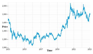
Figure 1: LBMA Gold closing price.

Influence on the price of gold has many factors, this paper chooses eight important factors. Data sources is come from investing.com. Table 1 shows the relevant data information, where SD is the standard deviation.

Table 1: Description of factors.

2.2. Factor Selection Method

2.2.1. Correlation Analysis

The relationship between LBMA gold and associated factors is quantified using the Pearson correlation coefficient (PCC) in this paper. The correlation becomes stronger when the absolute value of the correlation coefficient is greater. The degree of correlation in this paper is classified as follows: when \( |\text{r}| \) is 0-0.4, 0.4-0.6, 0.6-1.0, it is considered that the variables are weakly correlated, moderately correlated, and strongly correlated. The formula for the correlation coefficient is as follows:

\[ \text{ρ}_{\text{x,y}}\text{=}\frac{\text{E}[(\text{X-EX})(\text{Y-EY})]}{\text{ρ}_{\text{x}}\text{ρ}_{\text{y}}}\text{ (1)} \]

2.2.2. Causal Test

This paper employs Granger causality tests to assess the explanatory relationship between the influences and LBMA gold. In time series, the Granger causality test is defined as the variable X contributing to the explanation of the forecast of the variable Y. This implies that X is the Granger cause of Y if the joint forecast of the variable Y is superior to the forecast of Y alone. The formula of the Granger test is as follows:

\[ \text{F= }\frac{(\text{RSS}_{\text{R}}\text{-}\text{RSS}_{\text{UR}})\text{/q}}{\text{RSS}_{\text{UR}}\text{/}(\text{n-k})}\text{~}(\text{q,n-k})\text{ (2)} \] \[ \text{F= }\frac{(\text{RSS}_{\text{R}}\text{-}\text{RSS}_{\text{UR}})\text{/q}}{\text{RSS}_{\text{UR}}\text{/}(\text{n-k})}\text{~}(\text{q,n-k})\text{ (2)} \]

2.3. Model Selection

This article selects LSTM, Bi-LSTM, Multi-factor LSTM and Bi-Multi-factor LSTM to process the time series data of LMBA gold prices.

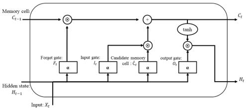
Figure 2: The schematic graph of the LSTM network.

The fundamental principle underlying the functioning of LSTM is the cell state. As illustrated in figure 2, the memory cell state \( \text{C}_{\text{t-1 }} \) of the previous moment initially discards irrelevant information (determined by \( \text{F}_{\text{t}} \) ), then incorporates data from the current input moment (determined by \( \text{I}_{\text{t}}\text{ } \) and \( \text{Ĉ}_{\text{t }} \) ), and finally outputs \( \text{C}_{\text{t}} \) and \( \text{H}_{\text{t}}\text{ } \) of the current moment. The following are relevant formulas of LSTM:

\[ \text{I}_{\text{t}}\text{=α}(\text{X}_{\text{t}}\text{W}_{\text{xi}}\text{+}\text{H}_{\text{t-1}}\text{W}_{\text{hi}}\text{+}\text{b}_{\text{i}})\text{ (3)} \]

\[ \text{F}_{\text{t}}\text{=α}(\text{X}_{\text{t}}\text{W}_{\text{xf}}\text{+}\text{H}_{\text{t-1}}\text{W}_{\text{hf}}\text{+}\text{b}_{\text{f}})\text{ (4)} \]

\[ \text{O}_{\text{t}}\text{=α}(\text{X}_{\text{t}}\text{W}_{\text{xo}}\text{+}\text{H}_{\text{t-1}}\text{W}_{\text{ho}}\text{+}\text{b}_{\text{o}})\text{ (5)} \]

\[ \text{Ĉ}_{\text{t}}\text{=tanh}(\text{X}_{\text{t}}\text{W}_{\text{xc}}\text{+}\text{H}_{\text{t-1}}\text{W}_{\text{hc}}\text{+}\text{b}_{\text{c}})\text{ (6)} \]

\[ \text{C}_{\text{t}}\text{=}\text{F}_{\text{t}}\text{(}\text{ C}_{\text{t-1}}\text{+ }\text{I}_{\text{t}}\text{( }\text{Ĉ}_{\text{t}}\text{ (7)} \]

\[ \text{H}_{\text{t}}\text{=}\text{O}_{\text{t}}\text{( tanh}(\text{C}_{\text{t}})\text{ (8)} \]

3. Results and Discussion

3.1. Data Processing

3.1.1. Missing Data

Due to the discrepancy in the dates between the LBMA gold price and the prices of the other eight factors, some data are incomplete. In this paper, the date of the LBMA gold price is employed as a reference point, and if the corresponding date of the LBMA gold price is not accompanied by date data for the other factors, the data for the other factors on the same date are excluded. In the event that data for other factors is absent on a given date, the data for the four adjacent days is employed to supplement the missing values. The processed data set presented in this paper comprises 2,608 LBMA gold closing prices and 20,864 related influencing factors.

3.1.2. Factor Selection

In this study, Granger causality tests are utilized to evaluate the explanatory connection between the influences ( \( \text{X} \) \( \text{X} \) ) and LBMA gold (𝑌). Before conducting the Granger Causal test, this paper employs first-order differencing and Augmented Dickey Fuller (ADF) test to ensure the stationarity of the data. From table 2, most of the original series is non-stationary. After passing the first order difference, for every variable, the p-value of ADF test is less than 1%, which indicates that the non-stationary hypothesis of this series can be disproved. ) and LBMA gold ( \( \text{Y} \) \( \text{Y} \)

Table 2: Results of the First-order Differencing and ADF Test.

Once the series had been assessed for stationarity, the Granger test was applied, the results of which are presented in the table 3. It shows that at the 1% significance level of the Granger test, the original hypothesis can be rejected if the p-value in "X is not the Granger cause of Y" is less than 1%, and the original hypothesis can be accepted if the p-value in "Y is not the Granger cause of X" is greater than 1%. This means that the variables satisfying these two conditions can be considered as Granger causes of LBMA gold price. On this basis, \( |\text{r}|\text{ } \) of the variables exceeding 0.6 were selected as input features for subsequent model development. That are Dow Jones industrial average and NASDAQ composite index.

Table 3: Results of the Correlation and Granger Test.

3.1.3. Normalization

From table 1, it is concluded that there is a large magnitude difference between the data, particularly in the case of the Dow Jones industrial average. The normalization process serves to mitigate the impact of disparate magnitudes of data on the performance of the prediction network, while simultaneously accelerating the gradient descent. Also, the values of the variables are transformed into the range [0,1] in order to facilitate the input of the subsequent LSTM model. Consequently, normalization is vital, and its formula is as follows:

\( \text{Xnew=}\frac{\text{X}_{\text{i}}\text{ - }\text{X}_{\text{min}}}{\text{X}_{\text{max}}\text{ - }\text{X}_{\text{min}}}\text{ (9)} \) \( \text{Xnew=}\frac{\text{X}_{\text{i}}\text{ - }\text{X}_{\text{min}}}{\text{X}_{\text{max}}\text{ - }\text{X}_{\text{min}}}\text{ (9)} \)

3.1.4. Data Segment

In this paper, the initial 85% of the data set is utilized as the training set for the models, with the remaining 15% serving as the test set for the model.

3.2. Forecasting

In this section, LSTM, Bi-LSTM, Multi-factor LSTM and Bi-Multi-factor LSTM are constructed to predict the closing price of the next day from the historical data of the past seven days. Therefore, the time step is seven and the input variable is a time step (t-1) feature. In essence, the input layer of LSTM and Bi-LSTM accepts the data of close prices of LMBA gold in the past seven days, while the input layer of the other two models also accepts the data of the past seven days of the two influencing factors (Dow Jones industrial average and NASDAQ composite index). Furthermore, the hidden size is set to 256 neurons and the output layer to one neuron. The loss function employed is Mean Squared Error (MSE), while the optimization algorithm is Adam. The model utilizes 50 epochs and a batch size of 64, with dropout incorporated into the two LSTM layers to prevent model overfitting.

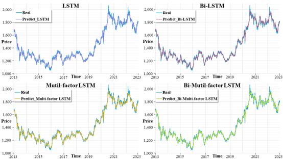
Figure 3: Forecast Results.

Figure 3 exhibits the forecast results. The number of predicted values for each model is 2,601, corresponding to the period from 11 January 2013 to 30 December 2022.

3.3. Model Evaluation

The performance of the model is evaluated using Mean Square Error (MSE) and Mean Absolute Error (MAE) metrics by quantifying the differences between predicted and true values. MSE measures the squared differences between predicted and true values, while MAE calculates the absolute differences between predicted values and target. The figure below illustrates the results of the model evaluation.

Table 4: Model Evaluation.

Table. 4 presents a comparison of the aforementioned models. The Bi-Multi-factor LSTM model has the smallest MSE and MAE, indicating that the smaller the difference between the predicted and true values, the more effective the model. Conversely, the Bi-LSTM model demonstrates superior performance compared to the original model. Its bi-directional processing of information enhances the accuracy of model estimation. However, when comparing the LSTM model with the Multi-factor LSTM, the authors observed that the MSE decreased while the MAE increased. This may be due to the effect of multivariate modelling on the distribution of prediction error. For instance, if the model reduces the frequency of large errors but increases the number of small errors, this could result in a decrease in MSE and an increase in MAE. As illustrated in the figure, the LSTM model exhibits suboptimal performance during the spike-back period. However, the model performance subsequently improves with the incorporation of the relevant factor variables.

The preceding analysis indicates that the Bi-Multi-factor LSTM model exhibits the most optimal prediction performance among the models under consideration. In the future, it may be possible to combine the Bi-Multi-factor LSTM model with other models for ascertaining whether the estimation accuracy can be further improved. Additionally, we observe that the introduction of correlated influence variables through methods such as correlation analysis and the Granger test almost enhances the prediction accuracy. However, the necessity of introducing correlated influence variables remains uncertain. It may enhance the model's predictive accuracy in the case of large errors, yet simultaneously increase the number of minor errors. This discovery aligns with the research conducted by Liu et al. [11]. Furthermore, it can enhance the explicitness of the model, which can facilitate comprehension of the rationale behind the model's prediction or decision-making process, thus facilitating further model debugging and optimization, as well as enhancing the decision-maker's capacity to make more informed decisions. Finally, the introduction of bi-directional networks can also enhance the precision of model predictions, which is consistent with the findings of Yurtsever [7].

4. Conclusion

This paper bases on LSTM model to predict the LBMA gold prices. It introduces bi-directional learning and multivariate analysis to assess the efficiency of the model. Ten years of data from 2013 to 2022 are analyzed to select the LBMA gold price and two related influences as input sources. The experimental results demonstrate that the introduction of multivariate analysis is more effective in dealing with outliers, but may increase the number of small errors. Furthermore, Bi-LSTM network may prove to be a more efficacious approach to enhancing the model's predictive accuracy.

At the same time, the experiment still has some limitations. Firstly, the quantity of input data and the number of selected influencing factors are insufficient. Secondly, the division of training and test set may also cause the model exhibiting overfitting. Thirdly, the use of the average value to supplement the missing values.

In future studies, in order to improve these, it is possible to introduce further correlation factors into the analysis and to expand the amount of data by including minute data or by extending the selected years. This will enable to increase a validation set, thus allowing further assessment of the extent of model learning. Furthermore, if the proportion of missing values is considerable, more complex approaches like the use of LSTM with an attention mechanism may be employed, which enables the focus on key information and the reduction of sensitivity to missing values.

References

[1]. Shafiee S, Topal E. An overview of global gold market and gold price forecasting[J]. Resources policy, 2010, 35(3): 178-189.
[2]. Baur D G, McDermott T K. Is gold a safe haven? International evidence[J]. Journal of Banking & Finance, 2010, 34(8): 1886-1898.
[3]. Rasekhschaffe K C, Jones R C. Machine learning for stock selection[J]. Financial Analysts Journal, 2019, 75(3): 70-88.
[4]. Guha B, Bandyopadhyay G. Gold price forecasting using ARIMA model[J]. Journal of Advanced Management Science, 2016, 4(2).
[5]. Liping X, Mingzhi L. Short-term analysis and prediction of gold price based on ARIMA model[J]. Finance Econ, 2011, 1.
[6]. Livieris I E, Pintelas E, Pintelas P. A CNN–LSTM model for gold price time-series forecasting[J]. Neural computing and applications, 2020, 32: 17351-17360.
[7]. Yurtsever M. Gold price forecasting using LSTM, Bi-LSTM and GRU[J]. Avrupa Bilim ve Teknoloji Dergisi, 2021 (31): 341-347.
[8]. Amini A, Kalantari R. Gold price prediction by a CNN-Bi-LSTM model along with automatic parameter tuning[J]. Plos one, 2024, 19(3): e0298426.
[9]. Xie H, Zhang L, Lim C P. Evolving CNN-LSTM models for time series prediction using enhanced grey wolf optimizer[J]. IEEE access, 2020, 8: 161519-161541.
[10]. DASH P, MISHRA J, DARA S. BIDIRECTIONAL CNN-LSTM ARCHITECTURE TO PREDICT CNXIT STOCK PRICES[J]. Journal of Theoretical and Applied Information Technology, 2024, 102(5).
[11]. Liu Y, Li L, Huang K, Wang Z, Wang C, Yang C. A Novel Zinc Price Forecasting Method Based on Multi-Factor Selection and LSTM Network. In2021 IEEE International Conference on Recent Advances in Systems Science and Engineering (RASSE) 2021 Dec 12 (pp. 1-8). IEEE.
Cite this article
Yan,H. (2024). Research on Gold Price Prediction Based on LSTM Modeling. Advances in Economics, Management and Political Sciences,94,202-210.
Data availability
The datasets used and/or analyzed during the current study will be available from the authors upon reasonable request.
Disclaimer/Publisher's Note
The statements, opinions and data contained in all publications are solely those of the individual author(s) and contributor(s) and not of EWA Publishing and/or the editor(s). EWA Publishing and/or the editor(s) disclaim responsibility for any injury to people or property resulting from any ideas, methods, instructions or products referred to in the content.
About volume
Volume title: Proceedings of ICFTBA 2024 Workshop: Finance in the Age of Environmental Risks and Sustainability
© 2024 by the author(s). Licensee EWA Publishing, Oxford, UK. This article is an open access article distributed under the terms and
conditions of the Creative Commons Attribution (CC BY) license. Authors who
publish this series agree to the following terms:
1. Authors retain copyright and grant the series right of first publication with the work simultaneously licensed under a Creative Commons
Attribution License that allows others to share the work with an acknowledgment of the work's authorship and initial publication in this
series.
2. Authors are able to enter into separate, additional contractual arrangements for the non-exclusive distribution of the series's published
version of the work (e.g., post it to an institutional repository or publish it in a book), with an acknowledgment of its initial
publication in this series.
3. Authors are permitted and encouraged to post their work online (e.g., in institutional repositories or on their website) prior to and
during the submission process, as it can lead to productive exchanges, as well as earlier and greater citation of published work (See
Open access policy for details).