1. Introduction

Today's culture brings influences and convergence to everything. Movies, radio, and magazines form a system called the "culture industry'', which was first mentioned by Theodor Adorno and Max Horkheimer in their book Dialectic of Enlightenment [1]. Hence, there is a trend of art appreciation occurring in recent years with huge evolution arising in related industries. This boom pushes up rapidly increasing popularity in art museums and obsession with art products.

This paper is going to focus on how the development of the art industry can be related to the economic cycle. Art is widely known as the diverse range of products of human activities involving creative imagination to express technical proficiency, beauty, emotional power, or conceptual ideas. The field of art is unique, encompassing both artistic and economic attributes. The keyword "cultural industry", or art industry, started emerging in various institutions [2]. The impacts on the art industry by economic development are meaningful to study as the importance of cultural diffusion increases among countries, just as Bourdieu viewed reputation, honour, and attention as symbolic capital that leverages both economic and social class advantages to individuals and groups [3].

Art product price is an important factor in measuring the health of art industry development, which can be quantified and considered as an indicator of demand for art products. Stein suggests that art products are a commodity with multiple attributes, both as a consumer durable and as a financial asset with a return on investment [4].

The main aim of choosing the topic for this project is to find out the relationship between art industries and the economic cycle. Firstly, the economic cycle’s impacts on the art industry will be analysed. Secondly, the changes in this industry brought by macroeconomic factors should also be the subject of this investigation.

After analysing the data, several trends have emerged. First, the positive impact of lower levels of economic development and higher levels of government expenditure on the arts industry is very clear.

Second, the development of the arts industry has little impact on most economic indicators. Third, the final impact of GDP on the art industry is uncertain, concluding that a positive correlation with ln (art prices) may be observed at the beginning of a small increase in GDP, while a quadratic pattern may be observed when the GDP index grows above a certain level and art prices fall. Further research may also be needed on the complex relationship between inflation and art prices.

By creatively using GDP and inflation as moderators, the study contributes to the existing literature by examining the relative strength of the direct and indirect link between art prices and the local economy, and by providing statistical evidence of the impact of art exhibitions on the economy. Furthermore, a sophisticated time-series model is used to scrutinise the two-way causal link between the economy and the art industry. The paper has clear managerial implications, such as enabling governments to better understand the importance of the cultural industries and to encourage the development of performing arts organisations and museums in moderation based on the relative strength of the parameters estimated in the model. Practitioners working in the arts industry will also benefit from a better understanding of the role that local economies, tourism and education play in improving the profitability of their organisation based on this paper.

2. Economic Cycle and Art Industry

In the 1980s, as the analysis of business cycles is proved, attention to this theory is brought to economists. According to early research, a business cycle is defined as a series of expansions and contractions that represent levels of aggregate output, employment, and many other factors and related processes. Of particular concern to economic watchers and observers are slight or severe declines in overall economic activity (recessions or depressions) in absolute terms [5].

Although the cultural sectors – arts, media, and design-related fields – possess relatively low employment levels, interest in these sectors is justified in both the popular press and scholarly research based on their remarkable growth rates and capacity to realize a host of secondary effects [6]. Cultural economy is defined as “the conception and production of products that have the function of entertaining, teaching, beautifying, and enhancing identity” [7]. Academic definitions and policies related to the cultural economy continued to evolve in response to the major economic, social, and political changes that began in the 1970s and 1980s, involving a range of industries, art-related mediums, and cultural products in different regions (eg. film, music and handcrafts).

The main part of the cultural industry covered in this paper is the traditional artwork market. It is believed that art has a high rate of appreciation and experiences cyclical booms and busts in the long term [8]. To investigate this fluctuation and its relationship with the economic cycle, the effects of both economic recessions and their economic impacts are involved.

2.1. The Effect of Economic Recession on the Art Industry

In particular, the decline in manufacturing and the restructuring of economies around business and consumer services, high technology, and electronic media, coupled with growth in professional employment and incomes, has led many governments to oversee urban cultural policy, where organizations are established to do so [9-11]. Political dynamics also come into play. Indeed, Britain's and Europe's emphasis on cultural development strategies derives from a more socially democratic politics, but ultimately an economic shift to meet the needs and demands of global finance [9,12].

However, with the onset of the global financial crisis and recession, the cultural economy may experience a dramatic rise in unemployment that fundamentally alters its structure and ability to deliver these purported spin-off effects. Given the attention many cities place on the cultural economy, it is important to examine how the cultural sectors fare following economic events.

2.2. Analysis of the Impact of the Recession on Art Market Prices

As Pratt observes, financial crises can change cultural and economic development patterns in three circumstances. First, the cultural economy relies on private consumption and has the potential to expand into other advanced sectors considered to support employment, namely finance and technology [7,13]. Employment in the cultural economy has also fallen significantly due to the financial crisis and its impact on housing spending and consumer spending, particularly in areas where financial speculation and foreclosures are highest. The result is "collapse". Areas with large cultural economies and concentrated industries such as finance, consumer services, and high-tech industries have shrunk most severely [11]. Although large cities enjoy the privilege of being cultural and economic leaders, they are also the most vulnerable to dramatic economic change. Researchers points out that the “interdependencies” and “external regional economies of scale and scope” that drive cultural economic spirals are “end market expansions” [7]. For example, if the market crashes, you can easily turn it around. Although the financial industry seems to be recovering rapidly from the collapse, the cultural industry, despite its dependence on finance, it is believed that cultural production plays a more central role in the overall economy and is no longer a subordinate position and proposes a "cultural production scenario" that currently occupies a core and dominant position in the economy [13]. "The driving force is economic structural adjustment. First, the cultural sector is thus virtually immune to recessions and has the potential to grow even in recessions. Its importance is increasing. "Many industries are also growing in importance. A third possible direction is a scenario of creative destruction, which involves phasing out products and ideas that have become obsolete because of the recession. This includes scenarios that intensify directing investment towards new products. In practice, companies would be willing to take risks, as many cultural economy companies are smaller, more adaptable towards different environments, and with lower start-up costs than the first scenario; the entrepreneurs benefit from new demand because initial costs are lower and there is a greater willingness to take risks.

Existing literature predicts that during economic downturns, occupations and regions that are highly dependent on finance, construction and consumption will experience greater job losses and higher unemployment rates. At the same time, however, given the importance of the cultural sector in the global economy, large, well-developed cultural centres are likely to maintain their advantage by their highly developed social and economic networks, labour forces and businesses. Smaller, less developed emerging centres of activity, on the other hand, are likely to decline because of greater economic pressures[6].

3. Data and Methods

To interpret further relationships between the art industry and the economic cycle, data analysis regarding art price and measurement of economic changes( percentage change in GDP from a year ago, GDP, CPI) are included in this paper. Both the Vector Autoregressive Model and the Multiple Regression Model will be included for analysing the two-way relationships between variables.

3.1. Data

For measuring the change in the economic cycle, in this paper, the percentage change in real GDP in the UK is used as a significant indicator measuring the economic cycle, acting as an independent variable, which data sources from the International Monetary Fund, accompanied by ln (art price index) as a dependent variable, for which the small values of change may be estimated as the variable’s percentage change. Art price indexes in the UK are included in the data set recorded by Artprice.com, which are calculated based on all Fine Art auction results (i.e. paintings, sculptures, drawings, photographs, prints, watercolours, etc.), using a base 100 in January 1998.

Other variables, the Consumer price index for the whole economy and service sectors, Government total consumption expenditure, and the UK GDP index, are sourced from the Organization for Economic Co-operation and Development and using a base 100 in January 1998, the same as the art price index. All data are recorded on a quarterly frequency from Q1 1998 to Q4 2021 for consistency.

3.2. Data Preprocessing

3.2.1. Autocorrelation Check

Autocorrelation is defined as similarity in three senses. First, a given time series has its backward version in the second case and a continuous time interval in the third case. In other words, autocorrelation is a measure of the relationship between the current value of a variable and its previously transmitted value.

Autocorrelation is considered as what should be entered if the calculation of the correlation between two different pairs of time-series values is required. For measuring the autocorrelation, simply calculate the original values and then calculate them again after different periods have elapsed. It should be noted that autocorrelation is ideal for finding trends and patterns in time series data that cannot be detected by other methods [14].

3.2.2. Seasonal Adjustment

Seasonal adjustments can be performed in two ways: multiplicative and additive. When the seasonal pattern is multiplicative, the magnitude of seasonal fluctuations increases proportionally over time. In other words, the seasonal effect reflects its percentage term, i.e., the absolute value of the seasonal change increases over time. This can be corrected by dividing each value in the time series by a seasonal index that represents the typical proportion observed in that season, i.e., by dividing each value in the time series by the seasonal index, which represents the percentage normally observed in that season.

As an alternative, multiplicative seasonal adjustment can be replaced by additive adjustment. A time series with constant seasonal variation is independent of the current mean of that time series. This is a candidate for additive seasonal adjustment. In additive seasonal adjustment, each value of a time series is adjusted by addition or subtraction. These values are absolute, often below or above the seasonal mean for a particular season of the year and are estimated from historical data. Seasonal addictive patterns are rarely found in nature. Series with natural multiplicative seasonal patterns can be transformed into series with additive seasonal patterns by performing a log transformation on the raw data [15].

3.3. Models

3.3.1. Interventional Analysis

Turning to the four main stages of intervention analysis apply to both long-term and short-term memory time series, they are intervention or anomaly detection, model estimation, model diagnosis and prediction. However, as discussed below, the main task of intervention analysis is to determine which interventions were implemented and which were not implemented. The model structure is as follows

\( {x_{t}}-u={z_{t}}+\frac{Θ(B)}{Φ(B)}{w_{t}} \) ,(1)

where \( Θ(B) \) is the moving average polynomial and \( Φ(B) \) is the autoregressive polynomial, and \( {z_{t}} \) is the intervention term.

Intervention effects need to be estimated with the basic ARIMA model in the series. These are the two components of the entire model. Various methods have been proposed. These following steps are required to be followed: First, use data before the intervention point to determine his ARIMA model for the series. Then, the ARIMA model is used to predict post-intervention values. Third, the difference between the actual and predicted values after the intervention is calculated. Fourth, the model was examined for differences from step 3 to determine intervention effects. The steps from step 4 onward vary depending on the software available. If there may be access to a suitable program, data may be used to estimate an overall model that combines the series ARIMA and the intervention model. Otherwise, only the variance from step 4 above can be used to estimate the scale and nature of the intervention [16].

3.3.2. Vector Autoregressive Model

Vector autoregressive (VAR) models are multivariate time series models at work that relate the observations so far of a variable to previous observations of that variable and previous observations of other variables in the system. They have traditionally been widely used in finance and econometrics as they provide a framework for achieving important modelling objectives such as data description, forecasting and structural inference. A VAR model is made up of a system of equations that represents the relationships between multiple variables. As an example, a VAR(1) in two variables can be written in matrix form as

\( [\begin{matrix}{y_{1,t}} \\ {y_{2,t}} \\ \end{matrix}]=[\begin{matrix}{c_{1}} \\ {c_{2}} \\ \end{matrix}]+[\begin{matrix}{a_{1,1}} & {a_{1,2}} \\ {a_{2,1}} & {a_{1,2}} \\ \end{matrix}][\begin{matrix}{y_{1,t-1}} \\ {y_{2,t-1}} \\ \end{matrix}]+[\begin{matrix}{e_{1,t}} \\ {e_{2,t}} \\ \end{matrix}] \) ,(2)

where \( {e_{i,t}}, i=1,2 \) denotes the error term.

A major advantage of the VAR model is that it can describe multidimensional causal relationships between multiple variables, helping researchers to obtain additional potential patterns for in-depth discussion and reference, and has practical applications in complex realistic settings therefore [17].

3.3.3. The Multiple Regression Model

This project’s multiple regression model adopted the log-log, quadratic, and linear functional form to investigate the effect of various independent variables on CFR, including the number of vaccinations, testing and other government actions.

\( {\hat{ln⁡(art price index)}_{i}} \) = \( {β_{0}} \) \( -{β_{1}}{ln{(CPI)}_{i}}+{β_{2}}{ CPI_{i}}-{β_{3}} {GDP_{i}}{ ^{2}}+{β_{4}}{ GDP_{i}}-{{β_{5}}ln({CPI service)}_{i}} \) + \( {ε_{i}} \) (3)

4. Results

4.1. The Two-way Causal Relationship between the Economic Cycle and the Art Price Index

The optimal lag length of 4 lags was included in this interventional analysis model. using the intervention analysis model with the smallest AIC value, which is ARMA(1,2,3,4), to explore how a direct intervention on the changes in art product price by local economic cycle, as shown in Table 1 and table 2, it is found that the percentage change in the UK real GDP from one year ago from 1999q1 to 2021q4 have an insignificant impact on the ln (art product price index) (p-value = 0.340), as shown in Table 3, representing that the direct causality between the economic cycle and art industry development may not be proved with the existing data.

Table 1: AIC and Log-likelihood of Different Lag Orders for Intervention Analysis Model.

Table 2: Granger causality tests

By using a vector autoregressive model among six variables, representing the economy, art industry, government spending, and inflation, on the one hand, it is found that the decrease in the development of the economy (a fall in ln(GDP)) and the rise in the government consumption affect the art industry, as shown in table 3. With the rising government consumption expenditure, there may be support for the industry, which causes an increase in the number of visitors to art museums, theatres, and cinemas. A bad condition of the economy may lead to favour of turning liquid money into assets, leading to higher demand for arts that preserve value as a form of investment.

On the other hand, the development of the art industry has little effect on most of the economic indicators. The development of this industry may only account for a small part of the economy, where most of the large economies, such as the UK, may rely little of their economic development on the cultural sector, although it is true that the cultural economy is transforming into a more diverse and significant part of the economy.

Table 3: Coefficient Estimation of Vector Autoregressive Model. (Only part of the results with art exhibitions as a dependent variable)

Note. Significance level: ‘*’ 0.1; ‘**’ 0.05; ‘***’ 0.01.

Turning to the multiple regression model, the one with its regression results is shown in Table 4, where the estimate is,

\( {\hat{ln⁡(art price index)}_{i}} \) = -2.901359 \( -0.0745304{ln{(CPI)}_{i}}+0.0016982{ CPI_{i}}- 0.0004818 {GDP_{i}}{ ^{2}}+0{1305529 GDP_{i}}-0.132425 {ln({CPI service)}_{i}} \) + \( {ε_{i}} \) (4)

Table 4: Multiple regression results measure the ln art price as the dependent variable. There are 94 observations. The R-squared value is 0.8936 and the adjusted R-squared value is 0.8875.

Looking at the square analysis of GDP, for every 1 trillion unit increase in the GDP, the ln(art price) changes by approximately a quadratic form, by the amount of \( - 0.0004818 ∆{GDP_{i}}{ ^{2}}+0{1305529 ∆GDP_{i}} \) . This suggests an uncertain final effect, where at the start of a rise in GDP (by a small amount), the ln(art price) experienced a positive relationship, while at around 130, the art price will fall with the higher GDP index. The quadratic pattern may be found in Figure 1.

Turning to the regression coefficient, this report finds that every 1% increase in the ln(CPI) decreases the ln(art price) by approximately 0.0745304. However, at the same time, the variable CPI gets a positive linear relationship with the art price index, with a coefficient of 0.0016982. Furthermore, a one-unit increase in ln CPI in the service sector decreases the ln(art price) by approximately 0.132425. Such a complex relationship may be found in Figure 2 and Figure 3.

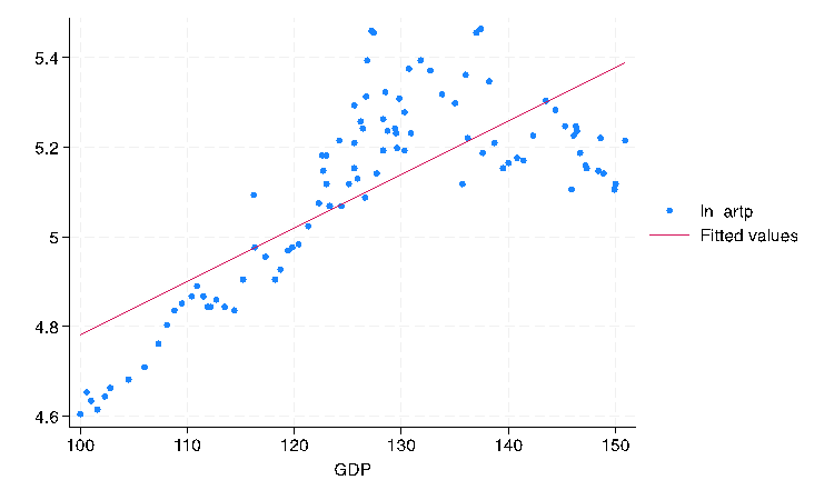
Figure 1: ln art price and GDP index

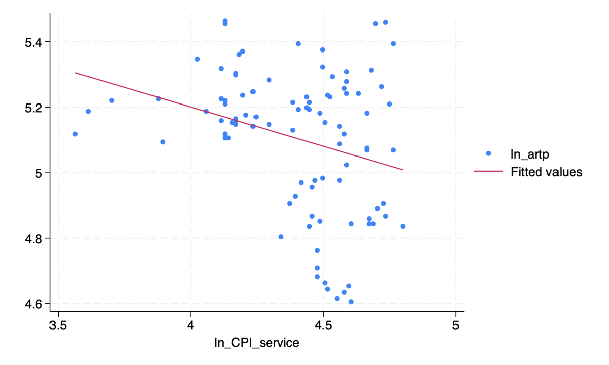
Figure 2: ln art price and ln CPI (service)

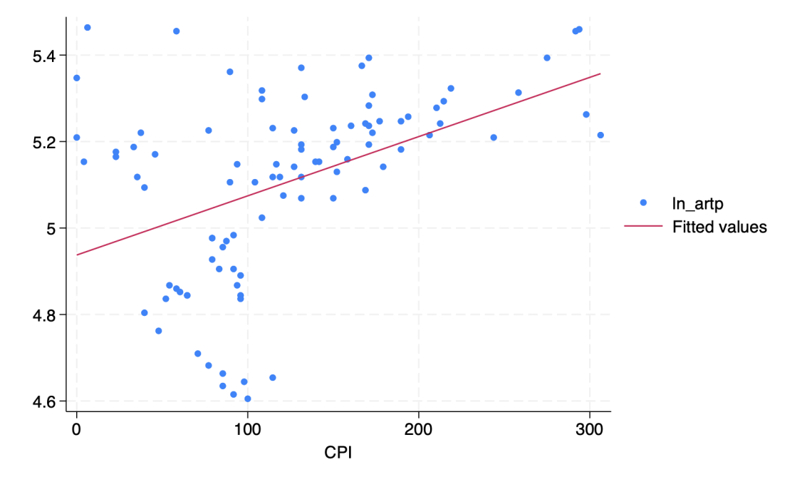
Figure 3: ln art price and CPI (total)

The \( {R^{2}} \) value of this regression model is 0.9760, which suggests that this is a higher proportion of the variation in CFR that is accounted for by the estimated equation. By conducting a two-sided hypothesis test on a 95% confidence interval,

\( {H_{0}} \) : \( {β_{i}} \) =0

\( {H_{1}} \) : \( {β_{i}} \) ≠0

All p-values are less than the significant value 0.05, rejecting \( {H_{0}} \) . This shows that data is well-fitted in this model.

However, there are some limitations. Firstly, the dataset was incomplete, which limited the analysis. The dataset and regression model could have been more accurate if more variable art product data related to dynamics (quality of art) and global-level data (art investment, government policies’ stringency towards the art industry) had been included. Furthermore, changes in the regressand may lag the effects in Inflation and GDP. Also, it may not conclude that there is a causal relationship between the art price and the economic cycle, and only a rough correlation could be included. In conclusion, a complex relationship between variables may be found, where more further investigations may be done to explain this trend.

5. Conclusion

This project aims to investigate the factors boosting the art industry. Firstly, the economic impact on the art industry was analyzed based on the intervention analysis model. Secondly, with the help of the vector autoregressive model, the two-way causal relationship between the art industry and the economic situation is explored.

The following results are obtained. Firstly, the decrease in the development of the economy and the rise in government consumption show a significant positive effect on the art industry. Secondly, the development of the art industry has little effect on most of the economic indicators. Thirdly, an uncertain final effect of GDP on the art industry is concluded, where at the start of a rise in GDP by a small extent may be a positive relationship between the ln(art price), while the art price will fall when the GDP index grows higher than a specific level, a quadratic pattern may be found. Also, the complex relationship between inflation and art prices may need further investigation.

This paper also contributes to the current literature by theoretically revealing the underlying mechanism of how the art industry can influence and be influenced by the development of the local economy. Moreover, the results can be well applied in decision-making by governments who seek to promote the local economy via art investment, or vice versa.

References

[1]. Adorno, T. (2022) "Frankfurt School: The Culture Industry: Enlightenment as Mass Deception". Retrieved from www.marxists.org.
[2]. Dong, C. (2012) “Analysis of Cultural Industry Development from the Perspective of Smile Curve Theory,” New Horizons, 6, 41–44.
[3]. Bourdieu, P. (2010) Distinction: A Social Critique of the Judgement of Taste. Taylor and Francis Group.
[4]. Stein, J. P. (1997) The Monetary Appreciation of Paintings. Journal of Political Economy, 85(5), 1021-1035.
[5]. Zarnowitz, V. (2006) Time Series Decomposition and Measurement of Business Cycles, Trends and Growth Cycles. Journal of Monetary Economics, Elsevier, 53(7), 1717-1739.
[6]. Carl, G., Michael, S. (2013) The Cultural Economy in Recession: Examining the US Experience. Cities, 33, 15-28.
[7]. Scott, A. (2007) Capitalism and Urbanization in a New Key? Social Forces, 85(4), 1465–1482.
[8]. Goetzmann, W.N. (1993) Accounting for Taste: Art and the Financial Markets over Three Centuries. American Economic Review, 83(5), 1370-1376
[9]. Bianchini, F. (1993) Remaking European cities: The Role of Cultural Policies. 21–57.
[10]. Grodach, C., Silver, D. (2012) The Politics of Urban Cultural Policy: Global Perspectives. London and New York: Routledge.
[11]. Hesmondhalgh, D. (2007) The Cultural Industries. London: Sage.
[12]. Oakley, K. (2012) A Different Class: Politics and Culture in London. The Politics of Urban Cultural Policy: Global Perspectives. London and New York.
[13]. Pratt, A. (2009) The Creative and Cultural Economy and the Recession. Geoforum, 40, 495–496.
[14]. Box, G. E. P., Jenkins, G. M., Reinsel, G. C. (1994) Time Series Analysis: Forecasting and Control. Upper Saddle River.
[15]. Ghysels, E., Osborn, D. R. (2001) The Econometric Analysis of Seasonal Time Series. New York: Cambridge University Press.
[16]. Krishnamurthi, L., Narayan, J., Raj, S. P. (1986) Intervention Analysis of a Field Experiment to Assess the Buildup Effect of Advertising. Journal of Marketing Research, 23(4), 337–345.
[17]. Kinal, T., Ratner, J. (1986) A VAR Forecasting Model of a Regional Economy: Its Construction and Comparative Accuracy. International Regional Science Review, 10(2), 113–126.
Cite this article
Xiong,Y. (2024). The Relationship Between the Development of the Art Industry and the Turnover of Economic Cycles. Advances in Economics, Management and Political Sciences,119,75-85.
Data availability
The datasets used and/or analyzed during the current study will be available from the authors upon reasonable request.
Disclaimer/Publisher's Note
The statements, opinions and data contained in all publications are solely those of the individual author(s) and contributor(s) and not of EWA Publishing and/or the editor(s). EWA Publishing and/or the editor(s) disclaim responsibility for any injury to people or property resulting from any ideas, methods, instructions or products referred to in the content.
About volume
Volume title: Proceedings of the 8th International Conference on Economic Management and Green Development
© 2024 by the author(s). Licensee EWA Publishing, Oxford, UK. This article is an open access article distributed under the terms and
conditions of the Creative Commons Attribution (CC BY) license. Authors who
publish this series agree to the following terms:
1. Authors retain copyright and grant the series right of first publication with the work simultaneously licensed under a Creative Commons
Attribution License that allows others to share the work with an acknowledgment of the work's authorship and initial publication in this
series.
2. Authors are able to enter into separate, additional contractual arrangements for the non-exclusive distribution of the series's published
version of the work (e.g., post it to an institutional repository or publish it in a book), with an acknowledgment of its initial
publication in this series.
3. Authors are permitted and encouraged to post their work online (e.g., in institutional repositories or on their website) prior to and
during the submission process, as it can lead to productive exchanges, as well as earlier and greater citation of published work (See
Open access policy for details).