1. Introduction

In the globalised financial market, stock index futures are not only used as an important tool for risk management, but also a hot topic of research in both academia and practice. [1]With the acceleration of international capital flows and the increasing integration of financial markets, the effectiveness of hedging strategies has become a common focus of investors and scholars.[2] The comparative analysis of the hedging efficiency of China CSI 300 Index (CSI 300) and Japan Nikkei 225 Index (Nikkei 225) futures contracts, as the representative financial derivatives of the two largest Asian economies, is of great theoretical and practical significance.

This paper aims to reveal the effectiveness of stock index futures hedging strategies and their differences in different market environments through empirical research. This study uses ordinary least squares (OLS), error correction model (ECM), value at risk (VaR) model[3], and measures the volatility of both to conduct an in-depth analysis of the trading data from January 1, 2023 to July 11, 2024.

The research questions focus on how to accurately measure hedging ratios and explore how differences between markets affect hedging effectiveness.[4] The study further examines how cross-market asset allocation can be optimised to reduce risk under volatile market conditions and assesses the performance of different hedging strategies in risk management. In particular, the flexibility and adaptability of hedging strategies are particularly important in the current context of increased uncertainty in financial markets.[5]

The significance of the study lies in the fact that it can not only provide international investors with more robust hedging strategies, but also provide new perspectives for understanding hedging mechanisms in different financial environments.[6] This paper also incorporates an analysis of how market volatility, investor sentiment and macroeconomic factors affect hedging efficiency. Through empirical analyses, this study expects to provide new evidence to support existing financial theories and provide valuable references for research and practice in related fields, especially in the current period when the global economy is facing many challenges.

2. Methodology

2.1. Data Source and Processing

In the article, the CSI 300 index is chosen as the underlying asset for hedging CSI 300 stock index futures, while the Nikkei 225 index is selected as the underlying asset for Nikkei 225 stock index futures. The experimental data covers a period from January 1, 2023 to July 11, 2024, totaling 349 trading days of closing prices. The data for both the CSI 300 index and CSI 300 stock index futures contracts are sourced from Invesco. To mitigate heteroskedasticity effects, all experimental data is transformed into natural logarithms. Price returns are also calculated as differences of variables using the following formulas:

\( ∆ln{{S_{t}}}=ln{{S_{t}}}-ln{{S_{t}}}-1 \) (1)

\( ∆ln{{F_{t}}}=ln{{F_{t}}}-ln{{F_{t}}}-1 \) (2)

Here, Equation (1) represents the formula for calculating spot price yields and Equation (2) represents futures price yields. In these equations, St denotes spot price on day t and St-1 denotes spot price on day t-1; Ft denotes futures price on day t and Ft-1 denotes futures price on day t-1.

2.2. Descriptive statistical analysis of yield data

Table 1: Descriptive statistics of futures price and spot price

According to the analysis of descriptive statistics, the average Nikkei 225 spot price return is -0.146 and the average Nikkei 225 futures price return is -0.129. Additionally, the average CSI 300 spot price return is 0.12, while the average CSI 300 futures price return is 0.125.

According to the figure 1 and Figure 2, the convergence between the Nikkei 224 Index spot and futures yields, showing a strong positive correlation with a correlation coefficient of 0.766 (p<0.001). Similarly, Figures 3 and Figure4 compare CSI 300 Index spot with its corresponding futures, revealing an even higher synchronization with a correlation coefficient as high as 0.946 (p<0.001), confirming a strong correlation between spot and futures markets.

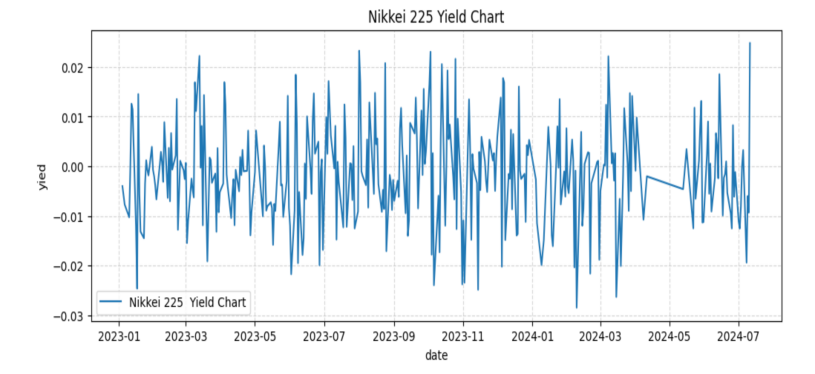
Figure 1: Nikkei 225 Spot Returns

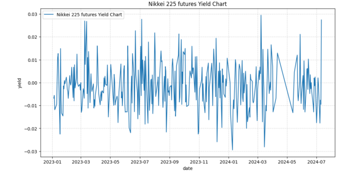
Figure 2: Nikkei 225 Futures Returns

Figure 3: CSI 300 Index Returns

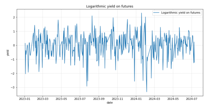
Figure 4: CSI 300 Futures Returns .

2.3. Smoothness analysis of yield data

To ensure the validity of subsequent regression analyses, we conducted ADF unit root tests on both NIKKEI300 and CSI300 futures and spot price returns. The results in Table 2 show that the t-values for NIKKEI300 are -18.81 and for CSI300 are -18.662, with corresponding p-values less than 0.01, rejecting the original hypothesis at the 1% significance level. This confirms that both return series contain unit roots and behave smoothly under the ADF test.

Similarly, Table 3 presents ADF test results for CSI300 futures and spot price yields, showing t-values of -17.834 for NIKKEI300 and -17.759 for CSI300, accompanied by very low p-values (<0.01). This again rejects the original hypothesis at the 1% significance level, proving that both markets' futures and spot price yield series exhibit stationarity under the ADF test.

Table 2: Nikkei 225 ADF Test Result

Table 3: CSI 300 ADF Test Result

2.4. Cointegration tests for spot and futures prices

To determine the long-term stable equilibrium relationship between spot price returns and futures price returns, we used the Engle-Granger two-step cointegration test.

\( ∆ln{{S_{t}}}=α+βln{{F_{t}}} \) (3)

The results of OLS regression analysis for the Nikkei 225 index show a significant fit with lnSt = -0.9 + 0.916lnFt (P<0.05, R²=0.877). Similarly, for the CSI300 index, the OLS regression analysis gives LnSt=0.087 + 0.989*LnFt with significant fit (P<0.05, R²=0.998). These results indicate a long-term stable equilibrium relationship between spot prices and futures prices.

Table 4: Regression results of least squares for NIKKEI 225 futures price and spot price

Table 5: Regression results of least squares for CSI 300 futures price and spot price

After obtaining the regression equation, the residuals are calculated as follows.

\( et=ln({S_{t}})-\hat{α}-\hat{β}ln({F_{t}}) \) (4)

After calculating the residuals, the residual series were tested for stationarity using the ADF unit root test. The results of the residual series are shown in Table 6 and Table 7.

(1) The t-value of NIKKEI 225 residual series in the ADF test is -8.473, with a significance p-value of 0.000*** at difference order 0, rejecting the original hypothesis. (2) The t-value of SCI300 residuals series in ADF test is -4.198 , with a significance p-value of 0.001*** at difference order 0, rejecting the original hypothesis.

The smooth time series indicates a cointegration relationship between NIKKEI225 and CSI300 spot price return and futures price return, allowing et to be used as a residual correction term for building a residual correction model

Table 6: Nikkei 225 residual series smoothness test results

Table 7: CSI300 residual series smoothness test results

3. Solving and analysing the hedging model

3.1. OLS Hedging Model

A least squares regression model is developed to estimate the hedging ratio, which is modelled as[2].

\( △ln{S_{t}}=α+β△ln{F_{t}}+{ϵ_{t}} \) (5)

The regression analysis using the OLS method shows that the R-squared value of the CSI 300 model is 0.894, significantly higher than that of the Nikkei 225 model at 0.521. In both models, the hedonic coefficient (ΔlnFt) is statistically significant and close to 1, indicating a strong positive correlation between changes in log futures returns and changes in log spot returns. The t-statistic of the hedonic coefficient for the CSI 300 model is 55.680, much higher than that of the Nikkei 225 model at 20.155, confirming robust parameter estimation for the CSI 300 model. The hedging ratio for the CSI 300 model is 0.9650, while for the Nikkei 225 model it is 0.7489. Both positive ratios are economically significant.

Table 8: Nikkei 225 Hedging results from the OLS model

Table 9: CSI 300 Hedging results from the OLS model

3.2. Vector autoregressive hedging model

The optimal lag between the CSI 300 index;CSI 300 stock index futures and the Nikkei 225 index; Nikkei 225 stock index futures needs to be found before building the VAR model.

The optimal lag of the VAR model is determined by using the information criteria AIC and SC. The optimal lag of the VAR model is determined by the information criteria AIC and SC.

The optimal lag of the Nikkei 225 VAR model was calculated by SPSS software to be 4 (see Table 10), which determined the establishment of the VAR (4) model; the optimal lag of the CSI 300 VAR model was 2 (see Table 6), which determined the establishment of the VAR (4) model

Table 10: Nikkei 225 Calculation Results of Optimal Lag Periods

Table 11: CSI 300 Calculation Results of Optimal Lag Periods

The basic idea of the model is as follows.

\( ∆ln{{S_{t}}}={α_{s}}+\sum _{i=1}^{p}{δ_{si}}∆ln{{F_{t-i}}}+\sum _{j=1}^{q}{θ_{sj}}∆ln{{S_{t-j}}}+{e_{st}} \) (6)

\( ∆ln{{F_{t}}}={α_{f}}+\sum _{i=1}^{p}{δ_{fi}}∆ln{{F_{t-i}}}+\sum _{j=1}^{q}{θ_{fj}}∆ln{{S_{t-j}}}+{e_{ft }} \) (7)

According to the vector autoregressive model, the hedging ratio between Nikkei 225 index and Nikkei 225 stock index futures is 0.9109 with a regression result of R2 = 0.655 and modified R2 = 0.646, indicating a good fit. The hedging ratio for CSI300 index and CSI300 stock index futures is 0.9428 with R2 = 0.935 and modified R2 = 0.934, also showing a strong fit. The results suggest that the CSI300 model performs better in explaining data variability and provides a more reliable hedging strategy compared to the Nikkei 225 model due to its higher R-squared values. Overall, the findings indicate that CSI300 stock index futures may be more effective in hedging risk relative to the spot index, making it a potentially valuable tool for practical applications.

Table 12: NIkkei 225 Hedging results by VAR model

Table 13: CSI 300 Hedging results by VAR model

3.3. Error Correction Model Hedging Model

The model underlying the error correction model is given by.

\( ∆ln{{S_{t}}}=α+ρ{e_{t-1}}+β∆ln{{F_{t}}}+\sum _{i=1}^{p}{δ_{i}}∆ln{{F_{t-i}}}+\sum _{j=1}^{q}{θ_{j}}∆ln{{S_{t-j}}+{e_{t}}} \) (8)

where et -1 is the error correction term, after regression by OLS.The results are shown in Table 14 and Table 15.

Table 14: Nikkei Hedging results by ECM model

Table 15: CSI 300 Hedging results by ECM model

By solving the error correction model, Nikkei 224R-squared: = 0.655 Adj. R-squared = 0.646, these two values are very close to 1, P = 0 < 0. 05 under F-test, indicating that the regression is well fitted, the model is significant, the hedging ratio is 0.9109 at this time. CSI 300R-squared: = 0.931 Adj. R-squared = 0.930, these two values are very close to 1, P = 0 < 0. 05 under F-test, indicating that the regression is well fitted, the model is significant, the hedging ratio is 0.9406 at this time. Very close to 1, F-test P = 0 < 0. 05, indicating that the regression is well fitted, the model is significant, and the hedging ratio is 0.9406 at this time.

Although the hedging ratios of the two models are similar, the error correction model of CSI 300 is significantly better than that of Nikkei 225 in terms of goodness of fit.

3.4. Comparison of Hedging Performance

In order to assess the performance of the hedging ratio using the minimum variance, assume a portfolio consisting of a long spot position of 1 unit and a short futures position of h units, with h being the optimal hedging ratio according to the different models. The hedging performance of the portfolio, ΔVH, is.

ΔVH = ΔlnSt - hΔlnFt ( 9)

\( ∆VH=∆ln{{S_{t}}}-h∆ln{{F_{t}}} \) (9)

The variance of the hedging portfolio performance is:

\( Var(∆VH)=Var(∆ln{{S_{t}}})+{h^{2}}Var(∆ln{{F_{t}}})-2hCov(∆ln{{S_{t}}},∆ln{{F_{t}}}) \) (10)

The degree of investment risk reduction is used to express hedging performance. The formula for calculating the degree of investment risk reduction (H) is as follows, and the final hedging performance results are shown in Table 15.

\( H=\frac{Var(∆ln{{S_{t}}})-Var(∆VH)}{Var(∆ln{{S_{t}}})} \) (11)

Table 16: Nikkei 225 and CSI 300 hedging performance by model

The Nikkei225 OLS model has an optimal hedging ratio of 0.7489 with a performance of 0.471933, while the VAR model has a ratio of 0.893 and a performance of 0.491677, and the error correction model has a ratio of 0.9109 with a performance of 0.486485. For the CSI300OLS model, the optimal hedging ratio is 0.9328 with a performance of 0.892875; for the VAR model, it is 0.9428 with a performance of 0.893402; and for the error correction model, it is 0.9406 with a performance of 0.893302. Python calculations show that the volatility of spot and futures returns for Nikkei225 index is higher than that for CSI300 index, indicating higher market risk for Nikkei225 index compared to CSI300 index due to its higher volatility in both spot and futures returns.

4. Conclusion

We observe that the Nikkei 225 demonstrates distinct hedging efficiency characteristics compared to its CSI 300 index. This disparity can largely be attributed to the heightened volatility of the Japanese market.

Firstly,elevated volatility implies increased uncertainty and risk exposure in the market, rendering it more challenging to forecast future price movements. Consequently, OLS, VAR, and ECM models may encounter greater difficulties in a more volatile market, thereby impacting their hedging efficiency. Additionally,ECM models may offer relatively better adaptability to high volatility by incorporating error correction terms to accommodate market dynamics. Conversely, the simplicity of the OLS model may result in suboptimal performance in a high volatility environment. The VAR model falls somewhere between these two extremes and is also influenced by market volatility.Moreover,Heightened volatility gives rise to heightened market risk, directly influencing hedging effectiveness. In a highly volatile market, even an optimal hedging ratio may not completely mitigate risk as market prices could fluctuate beyond the range predicted by the model.

References

[1]. Working, H. (1960). New concepts concerning futures markets and prices. *American Economic Review*, 52(2), 431-459.
[2]. Ederington, L. H. (1979). The hedging performance of the new futures markets. *Journal of Finance*, 34(1), 157-170.
[3]. Chung, Chu-Ying. (2023). A study on the hedging ratio of CSI 300 stock index futures and ETF funds. China Market, XX(23), 009.
[4]. Wang Jia, He Liuyang, Wang Xu. (2023). A study on multi-scale dynamic hedging of CSI 300 stock index futures based on EMD-DCC-GARCH. Financial Studies, 45(3), 123-145.
[5]. Yao Mu. (2023). Research on hedging efficiency of China's crude oil futures in the context of Russia-Ukraine conflict [Master's thesis, China University of Petroleum (Beijing)].
[6]. Xiao, Chao. (2014). Research on the hedging ratio of SZSE 100 ETF based on CSI 300 stock index futures [Master's thesis]. Northwestern University.
Cite this article
Liu,Y. (2024). Hedging Efficiency and Influencing Factors in Diversified Financial Markets — An Empirical Analysis Based on Futures of CSI 300 Index and Nikkei 225 Index. Advances in Economics, Management and Political Sciences,132,8-18.
Data availability
The datasets used and/or analyzed during the current study will be available from the authors upon reasonable request.
Disclaimer/Publisher's Note
The statements, opinions and data contained in all publications are solely those of the individual author(s) and contributor(s) and not of EWA Publishing and/or the editor(s). EWA Publishing and/or the editor(s) disclaim responsibility for any injury to people or property resulting from any ideas, methods, instructions or products referred to in the content.
About volume
Volume title: Proceedings of the 8th International Conference on Economic Management and Green Development
© 2024 by the author(s). Licensee EWA Publishing, Oxford, UK. This article is an open access article distributed under the terms and
conditions of the Creative Commons Attribution (CC BY) license. Authors who
publish this series agree to the following terms:
1. Authors retain copyright and grant the series right of first publication with the work simultaneously licensed under a Creative Commons
Attribution License that allows others to share the work with an acknowledgment of the work's authorship and initial publication in this
series.
2. Authors are able to enter into separate, additional contractual arrangements for the non-exclusive distribution of the series's published
version of the work (e.g., post it to an institutional repository or publish it in a book), with an acknowledgment of its initial
publication in this series.
3. Authors are permitted and encouraged to post their work online (e.g., in institutional repositories or on their website) prior to and
during the submission process, as it can lead to productive exchanges, as well as earlier and greater citation of published work (See
Open access policy for details).