1. Introduction

At the present stage of the human society development, a number of global-scaled problems gradually occur in succession. Intensification of international conflicts, threat of technological innovation to traditional industries, and rise of global trade tensions are all leading to greater uncertainty of the future, and predicting the future has become increasing important. For investors, policymakers, and financial analysts, prediction of financial indices is now an indispensable step before decision making. One of the crucial indices is the Standard and Poor’ s 500 index (S&P 500 index), which comprises the top 500 largest publicly traded companies in the U.S. It is a barometer of the overall health of the equity market and even the whole economy. Accurate forecasts of the index's future performance can guide investment strategies, risk management, and economic policy decisions. Given the S&P 500's significance in financial markets, robust predictive models are essential for navigating the inherent uncertainties of financial investing and economic planning.

Financial markets are inherently complex and volatile, characterized by numerous factors influencing price movements. According to Merton, this complexity necessitates advanced forecasting methods to capture the dynamic and often non-linear nature of stock market data [1]. Black and Scholes concluded that traditional methods, such as linear regression models, often fall short in accounting for the intricate patterns and dependencies present in financial time series [2]. To address these challenges, time series analysis has become a standard approach, providing frameworks to model and predict future values on the basis of historical data.

Among various time series models, the Autoregressive Integrated Moving Average (ARIMA) model stands out for its effectiveness in financial forecasting. Developed by Box and Jenkins in the 1970s, ARIMA is designed to handle data that is non-stationary, which is a common characteristic of financial time series [3]. The model's strength lies in its ability to integrate the autoregressive (AR) and moving average (MA) components, along with the differencing process (I), to capture a wide range of temporal dependencies and patterns in the data [4].

As suggested by Tsay, the ARIMA model is based on the principle that future values of a time series can be predicted by analyzing its past behaviors. This principle is particularly useful for financial data, where historical trends, cycles, and shocks can provide valuable insights into future movements [5, 6]. By applying ARIMA to the S&P 500 index, analysts can leverage historical data to forecast future values, potentially enhancing investment decisions and economic forecasts.

The efficacy of ARIMA models in predicting stock market indices have been demonstrated by several studies. For example, a study by Chen highlighted the model's capacity to provide reliable forecasts for the S&P 500, emphasizing its adaptability to various market conditions [7]. Similarly, Kim provided a detailed analysis of ARIMA’s predictive performance, revealing its strengths in capturing long-term trends and short-term fluctuations in the S&P 500 index [8]. These findings underscore ARIMA’s robustness in financial time series analysis, making it a valuable tool for investors and analysts [9].

The relevance of ARIMA in financial forecasting is further supported by its extensive application in various research contexts. For example, the work of Enders demonstrated how ARIMA models can be employed in macroeconomic forecasting, while Hyndman and Athanasopoulos provided a comprehensive guide on the practical implementation of ARIMA models [10]. These studies reinforced the model's applicability across different domains, including stock market prediction.

Previous studies have clearly demonstrated that predicting the S&P 500 index is of paramount importance due to its impact on investment decisions and economic policy. The ARIMA model offers a robust framework for prediction based on historical data, leveraging its ability to account for trends and patterns in financial time series. The model is a powerful tool in financial forecasting, as evidenced by numerous studies and practical applications. This essay will explore the application of the ARIMA model in predicting future values of the S&P 500 index, examining its effectiveness, limitations, and the insights gained from past data to provide a comprehensive understanding of its role in financial analysis.

2. Methods

2.1. Data Collection

By accessing the S&P Global’s official website, this paper collected the closing prices for the last day every year from 1957, the year in which the S&P 500 index was established, to 2023. Fluctuation of the index can be attributed to a range of economic and political factors, including changes in GDP and unemployment rate, changes in policies, geopolitical events, and market sentiment.

Figure 1 shows the S&P 500 index from 1957 to 2023. Although the global economy as a whole has been growing in recent decades, resulting in an overall upward trend of the index, there are still random fluctuations due to unpredictable events. There are two major periods of rapid growth: from 1995 to 2000 and from 2010 to 2023. Years of major decline include 2008, because of the global financial crisis, and 2022, due to the spread of COVID-19.

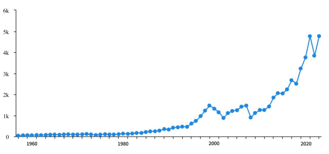
Figure 1: S&P 500 index.

2.2. Model Selection

The model used in this research is the Autoregressive Integrated Moving Average (ARIMA) model. As a popular statistical method used for time series forecasting, the ARIMA model analyzes past data and predicts the future. The model has three components. The Autoregressive (AR) part models the time series as a function of its own previous values; the Integrated (I) part differentiates the time series data to make it stationary, giving the series constant statistical properties; the Moving Average (MA) part models the relationship between the observation and residue errors and accounts for random variations in the data series.

3. Results and Discussion

3.1. Data Processing

A premise of the ARIMA model is that the input series must be stationary.

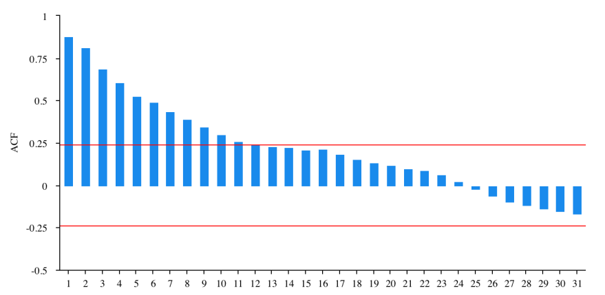
Figure 2: ACF plot for zero-order difference.

Figure 2 demonstrates the original data series, which is a non-stationary sequence and has strong auto-correlation, thus it has to be differentiated before being used to construct the model.

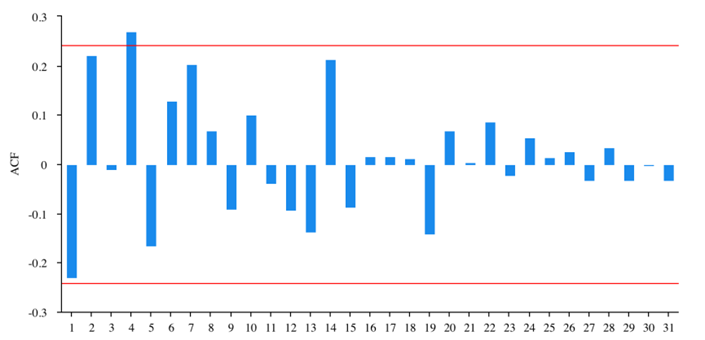
Figure 3: ACF plot for first-order difference.

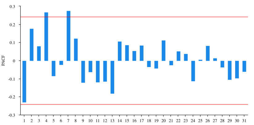
Figure 4: PACF plot for zero-order difference.

Figure 3 and figure 4 show the results of the first-order difference. By performing an ADF test on the results the author finds the p-value is 0.869, which means the series is still non-stationary.

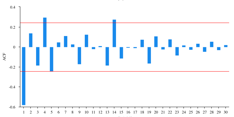
Figure 5: ACF plot for second-order difference.

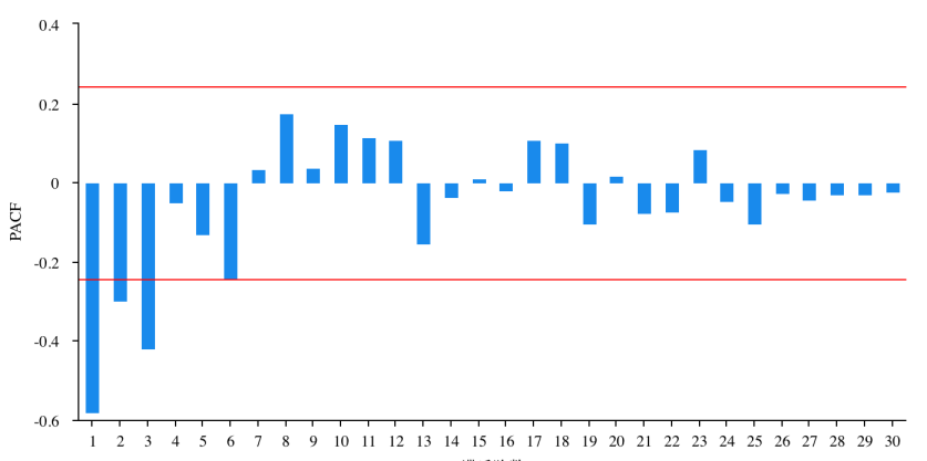
Figure 6: PACF plot for second-order difference.

Figure 5 and figure 6 show the results of the second-order difference. The results of the ADF test shows the p-value is 0.000, indicating that the series after differentiation is stationary. Therefore, it can be concluded that the optimal for d in the ARIMA model is 2.

3.2. Model Evaluation

A model can be evaluated by examining the deviation between its predicted values and the actual values: a smaller deviation indicates higher level of accuracy and better performance of the model. Another criterion is simplicity: simpler models are considered better than complicated models.

There are three variables in the ARIMA model: p, d, and q, corresponding to AR, I, and MA respectively. In part 3.1, the author has chosen the optimal d value, so he following step is to determine p and q.

The three metrics chosen are Akaike Information Criterion (AIC), Bayesian Information Criterion (BIC) and Root Mean Squared Error (RMSE). Both AIC and BIC assess the balance between model fit and complexity, with lower values indicating a better model, and BIC tends to favor simpler models more than AIC. While RMSE directly measures the average magnitude of errors between predicted and observed values, and lower values indicate a better fit of the model to the data.

Table 1: Model Evaluation.

From Table 1 it can be seen that ARIMA (1,2,2) gives the lowest AIC and BIC value. The RMSE values of ARIMA (4,2,2), (4,2,1), (3,2,2), (2,2,2) and (1,2,2) are all small and also close to each other. Therefore, this essay considers ARIMA (1,2,2) as the best model for analyzing and predicting the S&P 500 index.

3.3. Model Prediction

The following part makes a prediction of the S&P 500 index for the next 12 years (Figure 7).

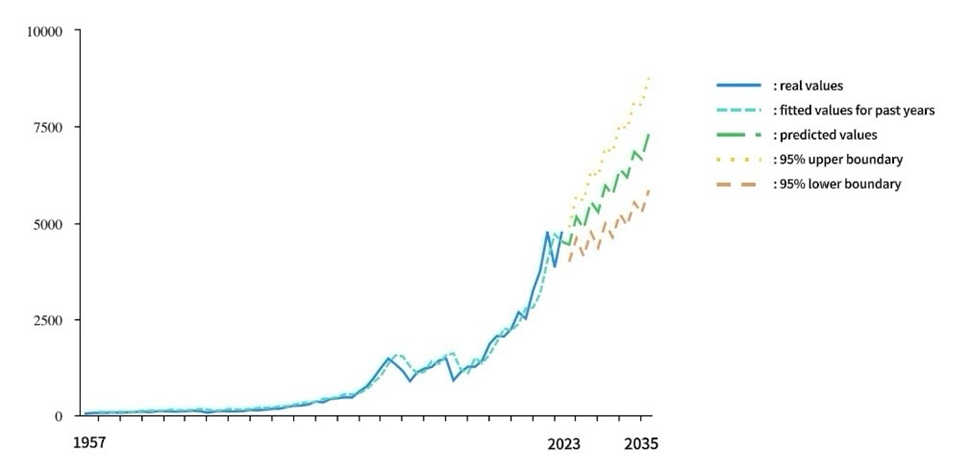
Figure 7: Prediction from ARIMA (1,2,2).

Table 2: Predictions from ARIMA (1,2,2).

As shown in Figure 7, the blue curve shows the real values from 1957 to 2023, and the blue-green curve shows the fitted value for past years. The green, yellow, and orange dotted curve represents the predicted value, the 95% upper boundary, and the 95% lower boundary respectively. The real values demonstrate an overall upward trend with three major periods of decline: 1999-2002 corresponds to bombing Yugoslavia and 911, 2007-2008 corresponds to the financial crisis, and 2021-2022 corresponds to the spread of Corona virus. Table 2 shows the predicted values, which demonstrates an upward trend with regular fluctuations.

3.4. Check Residuals

The residues of an accurate ARIMA model should be white noises.

Table 3: Ljung-Box test.

Table 3 shows the results of the Ljung-Box test. Since the p-value of Q6 is 0.434, bigger than 0.05, this paper concludes that the residues from ARIMA (1,2,2) are white noises.

3.5. Result Analysis

The predicted results from ARIMA (1,2,2) fluctuate around a linear upward trend. Though the results have passed theoretical tests, the predicted values are still likely to deviate from the real future value. The first reason for the deviation lies in the change of the overall growing rate in 1994. Before 1994 the S&P 500 index grows in a low rate, while after 1994 the rate significantly increased. Thus, if only the data after 1994 is taken into account, the prediction results from the model may show a faster rate of increase and be more accurate. However, this may lead to omission of information and loss of data integrity. The second reason lies in the unpredictability of future events. As discussed above, the historical trend has three major periods of decline, each corresponding to important historical events. Whereas significant evens are unpredictable, causing uncertainty in future fluctuations. The increase and decrease of the index will not be regular as shown by the prediction, instead it will be random.

4. Conclusion

This essay makes a prediction on the future S&P 500 index using the ARIMA model based on data from 1957 to 2023. Differential processes are carried out to stabilize the data set and the second-order difference is determined as the most appropriate one. Using AIC, BIC, and RMSE values as criteria, this essay evaluates models with different coefficients and chooses ARIMA (1,2,2), which concluded that the index will continue to increase with fluctuations.

The prediction results do provide people with an insight into the future, but there will be deviations between the real values and the predicted values due to uncertainty and randomness of future events. Today’s unstable international situation, demonstrated by major events such as the Russo-Ukrainian War and the Israeli-Palestinian Conflict, even makes the index more unpredictable. Thus, the results from the model may be further improved by taking the realistic conditions into account.

References

[1]. Merton, R.C. (1980) On Estimating the Expected Return on the Market: An Exploratory Investigation. Journal of Financial Economics, 8(4), 323-361.
[2]. Black, F. and Scholes, M. (1973) The Pricing of Options and Corporate Liabilities. Journal of Political Economy, 81(3), 637-654.
[3]. Box, G.E.P., Jenkins, G.M. and Reinsel, G.C. (2008) Time Series Analysis: Forecasting and Control (4th ed.). Wiley. Hamilton, J.D. (1994) Time Series Analysis. Princeton University Press.
[4]. Hamilton, J.D. (1994) Time Series Analysis. Princeton University Press.
[5]. Tsay, R.S. (2010) Analysis of Financial Statements (2nd ed.). Wiley.
[6]. Chen, N.F. (2017) Forecasting S&P 500 Returns Using Time Series Models. Journal of Financial Economics, 124(2), 295-315.
[7]. Kim, J. (2019) Predictive Performance of ARIMA Models for the S&P 500 Index. Journal of Financial Research, 42(1), 1-20.
[8]. Pagan, A. and Schwert, G.W. (1990) Alternative Models for Conditional Stock Volatility. Journal of Applied Econometrics, 5(2), 265-280.
[9]. Enders, W. (2004) Applied Econometric Time Series (2nd ed.). Wiley.
[10]. Hyndman, R.J. and Athanasopoulos, G. (2018) Forecasting: Principles and Practice. OTexts.
Cite this article
Wang,Y. (2024). Prediction of the Standard and Poor’s 500 Index Based on ARIMA Model. Advances in Economics, Management and Political Sciences,136,43-50.
Data availability
The datasets used and/or analyzed during the current study will be available from the authors upon reasonable request.
Disclaimer/Publisher's Note
The statements, opinions and data contained in all publications are solely those of the individual author(s) and contributor(s) and not of EWA Publishing and/or the editor(s). EWA Publishing and/or the editor(s) disclaim responsibility for any injury to people or property resulting from any ideas, methods, instructions or products referred to in the content.
About volume
Volume title: Proceedings of the 3rd International Conference on Financial Technology and Business Analysis
© 2024 by the author(s). Licensee EWA Publishing, Oxford, UK. This article is an open access article distributed under the terms and
conditions of the Creative Commons Attribution (CC BY) license. Authors who
publish this series agree to the following terms:
1. Authors retain copyright and grant the series right of first publication with the work simultaneously licensed under a Creative Commons
Attribution License that allows others to share the work with an acknowledgment of the work's authorship and initial publication in this
series.
2. Authors are able to enter into separate, additional contractual arrangements for the non-exclusive distribution of the series's published
version of the work (e.g., post it to an institutional repository or publish it in a book), with an acknowledgment of its initial
publication in this series.
3. Authors are permitted and encouraged to post their work online (e.g., in institutional repositories or on their website) prior to and
during the submission process, as it can lead to productive exchanges, as well as earlier and greater citation of published work (See
Open access policy for details).