1. Introduction

The real estate market is a crucial segment which indicates the overall economic development in a country. It highlights the ongoing urban expansion and changes in the social dynamics of the population and their living conditions. The development of the housing or the real estate market also mirrors the economic growth in a country. As a result, accurate price prediction of properties is a crucial matter because it helps government in formulating policies and regulatory frameworks which ensures a healthy and the long-term development of the sector [1]. In the contemporary literature, the housing market in Melbourne has garnered significant attention over the past decade due to extensive changes in the price level and ongoing volatility in the market. A wide range of literature suggests that the market experienced several fluctuations in the property prices due to different macroeconomic indicators like changes in the level of interest rates, government expenditure, population, demand for housing, and investment level [2]. However, another strand of literature suggests that the house prices are also influenced by internal factors like the characteristics of the properties and the locality of the houses [3][4]. Although, many studies have employed machine learning models in predicting the house price in Melbourne, it is critical to evaluate the house prices using a different set of models and identify if the same results are obtained. Through precise prediction of the property price, the decision-making of investors, individual buyers, and the urban planning authorities of the country can be enhanced, while considering market stability and affordability concerns.

Real estate price prediction models are crucial for offering insights into market patterns, assisting players in making educated decisions. Some of the conventional forecasting methods frequently utilize macroeconomic data, like Gross Domestic Product (GDP), inflation rates, and employment levels, to project future property values. Although these methods possess value, they often neglect the detailed, property-specific elements that substantially influence price fluctuations [5]. The unique attributes of different properties—such as bedroom count, proximity to services, and land size—are essential in assessing their market value. This exclusion requires the implementation of more sophisticated and comprehensive models, such as the hedonic price model, capable of incorporating these intricate properties [3][4]. In other words, the internal factors associated with the property are the better indicators of the house price and can better assist with the decision-making of property purchase as compared to the volatile macroeconomic indicators.

In line with the previous argument, the focus of the current paper lies with the hedonic pricing theory, that was initially proposed by Rosen [6]. The theory posits a method to analyse the price of a property by breaking it down into its individual features. This model suggests that the price of a good, such as a house, is affected by various aspects that independently contribute to its overall value. The utilization of hedonic models in the real estate sector is especially pertinent due to the infrequent uniformity of home prices. Rather, they vary according to structural characteristics (e.g., the dimensions and state of a residence) and locational elements (e.g., nearness to core business districts, educational institutions, or transit nodes) [7]. In other words, the physical characteristics or elements of the property collectively determine its overall value, and the hedonic method allows researchers to discern and measure the individual influence of each attribute on the ultimate price which further guides towards a better decision-making regarding the purchase of the properties in regions like Melbourne – which is also subject to high price fluctuation due to extensive demand in the market.

In this paper, Melbourne housing marketing is a key focus of interest and it is suitable to perform hedonic price model as the region comprise high-density apartments. The city's real estate landscape is complex, influenced by various socio-economic, topographical, and structural elements. In contemporary literature, it is observed that proximity factor is a crucial indicator in determining the price of the properties. For example, proximity to central business district and other amenities can positively contribute to the price and value of the property. On the other hand, availability of rooms and the size of land are the positive predictors of prices in the various regions [8][9]. The consideration of these factors suggests that physical and the spatial characteristics of the property can significantly determine the value of properties.

In term of the modelling approach, some studies suggest that prediction accuracy measures like root mean squared error (RMSE) and mean absolute error (MAE) are useful while R-squared metrics is useful in gauging the explanatory power of the model. Due to a significant range of variables, it is possible that regression model renders high explanatory power with significant predictors. However, simple linear models fail to capture market volatility which eventually leads to high prediction errors and low accuracy. Therefore, calculation of prediction accuracy measures like RMSE is important to complement the significance of observed adjusted R-square values [10][11]. In other words, the development of regression models with a wide range of house characteristics and features can lead to promising explanatory power of the model. However, it is also critical to consider the predictive accuracy of the models by computing the relevant statistics so that more realistic and acceptable results are obtained with less violation of OLS assumptions.

In hedonic price model, physical and other associated attributes of the properties are considered to estimate and predict property prices. In order to implement the model, the current research paper utilizes data from Kaggle – an open-source platform of data. The primary aim of the study is to determine the determinants or the factors influencing housing price in Melbourne region of Australia. As a result, the key focus of interest lies in the property-specific attributes, like the location of the house or the property, home type, total number of rooms, proximity to the CBD, total size of the land, and council area. In many studies, the researchers have advocated the effectiveness of the hedonic model by suggesting that it highlights the most significant factors considered by the people or the potential buyers while purchasing a property [7][12]. In some studies, it is suggested that closeness to specific locations like educational institutes, market, and other venues enhances the spatial significance of the properties which in turn aids in increasing the overall price [13]. However, understanding the influence of these factors on the property prices can be a complex matter of interest which requires strict considerations of robust models for prediction purposes. Therefore, the key objectives of the current paper are:

• To determine the most significant factors affecting house price in Melbourne, using historical data.

• To identify a robust model with high prediction accuracy in terms of forecasting house prices in Melbourne.

In order to fulfill the key objectives of the research, the paper initially discusses the methodology employed to analyse the data whereby key steps of data collection, processing, and analysis are outlined. The next section of the paper highlights the key findings from the models and overall exploratory data analysis. The subsequent section of the paper critically highlights the conclusion and future research implication, with a brief discussion of the limitation of the analysis.

2. Methodology

In this section of the paper, data collection, processing and analysis steps are outlined and the subsequent methods are discussed. The purpose of the chapter is to aid the researchers in understanding the steps taken to accomplish the analytical objectives of the paper. Initially, data source and dataset are critically discussed, followed by pre-processing methods involved to correct and normalize the variables. The next segment of the section outlines the key methods involved in exploratory and regression analysis, followed by a discussion of model accuracy measures.

2.1. Data Collection and Sources

The data used in this paper is sourced from Kaggle which is an open-source collaborative platform for researchers and developers to share or access code and data for research purposes or learning purposes [14]. The current paper uses Melbourne Housing Prices data whereby the data involves information on 34,858 properties from 9^th March 2016 to 5^th December 2018. Table 1 suggests that some of the variables in the data are numerical and some of them are categorical, which also adds diversity in the analysis.

Table 1: Data Description of Melbourne Housing Price which is collected from 9^th March 2016 to 5^th December 2018 from Kaggle open-source database

2.2. Data Preprocessing

2.2.1. Handling Missing Data

• Imputation: In order to deal with the missing values regarding numerical variables, median imputation is applied whereby the median of the variable is replaced with the missing values. This method is applied on several numerical variables in the dataset with missing values like land size and building area.

• Categorical variables: Due to non-numeric nature of certain variables like council area and region names, missing or unknown entries are replaced with NA or Unknown categories so that exclusion bias is controlled along with outlier issue.

2.2.2. Encoding Categorical Variables

The categorical variables such as Type, Suburb, and Council Area were converted into numerical values by dummy encoding, sometimes referred to as one-hot encoding. In machine learning, this method is employed to transform the categorical variables so that a large set of numerical variables is obtained. This method is more flexible while working with advance and complex models to forecast or predict a dependent variable [15]. This method generates binary columns for each category, enabling the regression model to include the influence of each categorical variable without enforcing any false ordinal hierarchy. For example, the "property type" variable was split into binary variables (house, apartment, townhouse, etc.).

2.2.3. Normalizing Continuous Variables

Real estate data typically contains continuous variables with varying scales which may leads to biased estimates, if not managed properly. In this sample dataset, land sizes ranged from 100 to over 1,000 square meters. Therefore, min-max normalization was applied to ensure uniformity in the models while scaling continuous variables between 0 and 1 [16]. The application of the transformation prevented the inclusion of disproportionately scaled variables in influencing the model.

2.2.4. Outlier Detection and Treatment

In this research, boxplot is used to visualize the prevalent outliers in the dataset so that appropriate transformations can be applied while controlling for excessive volatility [17]. The rationale of retaining and normalizing the values instead of removing the entries with volatile values is to ensure that proper analysis is conducted without exclusion bias. In most cases, removal of rows with missing and extremely high values are removed which leads to bias in the results due to non-inclusion of the core information.

2.2.5. Exploratory Data Analysis (EDA)

Once the data was pre-processed, an extensive EDA was conducted using R to explore variable relationships and guide feature selection. The following techniques were employed:

• Correlation Matrix: A correlation matrix was used to examine the relationships between continuous variables. Variables such as distance from the CBD and land size showed moderate correlations with property prices, indicating their relevance.

• Scatter Plots and Boxplots: These visualized the relationships between property price and continuous variables (land size, building area, distance to CBD). The boxplots highlighted the price distributions across different categorical variables (property type, council area).

• Histograms and Density Plots: These were used to assess the distribution of property prices, which exhibited positive skewness due to high-end properties. A logarithmic transformation was applied to normalize this distribution for better model performance.

2.2.6. Model Development

2.2.6.1. Multiple Linear Regression

The main model used in this study is Multiple Linear Regression (MLR). It estimates the relationship between the dependent variable (property price) and several independent variables (property characteristics), providing an interpretable framework for hedonic price modelling.

The general form of the MLR equation is:

\( Y= α+β1X1+β2X2+…+βnXn+ϵ \) (1)

Where:

• Y is the dependent variable (property price),

• X1,X2,...,Xn are the independent variables (property characteristics),

• α​ is the intercept,

• β1, β2,...,βn are the coefficients of the independent variables,

• ϵ is the error term.

The coefficients βi represent the effect of a one-unit change in the independent variables on property price, holding other variables constant.

2.2.6.2. Feature Selection

Feature selection was performed using the following techniques:

• Correlation Analysis: Variables with low correlation to property prices were considered for removal.

• Variance Inflation Factor (VIF): To detect multicollinearity, VIF was calculated for each independent variable. Variables with a VIF greater than 10 were considered for removal or transformation.

2.2.6.3. Ridge and Lasso Regression

Ridge regression and Lasso regression were implemented to handle multicollinearity and overfitting issues by imposing penalties on the size of the regression coefficients. These regularization techniques helped shrink irrelevant variables toward zero:

• Ridge Regression: Adds a penalty proportional to the sum of squared coefficients.

• Lasso Regression: Adds a penalty proportional to the absolute values of the coefficients, leading to sparse solutions by effectively performing feature selection.

The tuning parameter λ was optimized through cross-validation.

2.2.7. Model Validation

2.2.7.1. Train-test Split

The dataset was divided into a training set (80%) and a test set (20%) to evaluate the model's performance. The training set was used for model development, while the test set assessed its generalizability.

2.2.7.2. Cross-validation

K-fold cross-validation (with k=5) was employed to ensure model robustness. This technique divided the training set into five subsets, using four for training and one for validation, repeating the process until each subset had served as a validation set.

2.2.7.3. Performance Metrics

In the contemporary research, many scholars leveraged machine learning models to predict house prices. Some of the common indicators are R-square, adjusted R-square, RMSE, MAE, and other prediction accuracy measures [10][11]. The current research utilizes R-square and RMSE to gauge the explanatory and prediction accuracy of the selected models:

• Root Mean Squared Error (RMSE): Assesses the average magnitude of prediction errors, with greater emphasis on larger errors.

• Mean Absolute Error (MAE): Measures the average absolute difference between predicted and actual values, offering a straightforward error metric.

• R-squared (R²): Indicates the proportion of variance in the dependent variable explained by the independent variables, with a value closer to 1 representing a better fit.

3. Results and Findings

3.1. Summary Statistics

Table 2 suggests the categorical variables within the data associated with Melbourne House prices. The Suburb variable indicates that homes are dispersed among multiple Melbourne suburbs, with Reservoir being the most commonly reported, comprising 844 properties. Suburbs such as Bentleigh East (583) and Richmond (552) closely behind. This suggests that these regions are likely important residential centers in Melbourne, drawing increased listings due to heightened demand or property availability. The substantial quantity of suburbs categorized as "Other" (31,435) illustrates the dataset's extensive geographic scope, encompassing properties from diverse regions and providing a comprehensive perspective on Melbourne’s real estate market. In terms of the Type, it is observed that Houses (h) comprise the majority, with 23,980 listings, signifying that detached homes are the predominant property type in the dataset. Units (u), presumably denoting apartments, account for 7,297 entries, and Townhouses (t) comprise 3,580 items. This indicates that houses are the predominant property type, succeeded by units and townhouses. The predominance of houses suggests that Melbourne's housing market prefers single-family residences, although townhouses and apartments also play a role in the urban residential environment.

Table 2: Summary Statistics: Categorical Variables

Table 3 suggests summary statistics associated with the numerical variables in the dataset where the measures of central tendencies and dispersion are highlighted. The over property price ranges from a minimum of $85,000 to a maximum of $11.2 million, indicating the diversity of property values across different suburbs and types. The median price of $870,000 suggests that the typical property in the dataset is priced within this range, while the mean price of $1,010,838 indicates that higher-end properties may skew the average upward. The interquartile range between $695,000 (1st quartile) and $1,150,000 (3rd quartile) shows that the middle 50% of property prices fall within this bracket, representing moderate to high-value properties. The median number of rooms is 3, with the mean slightly higher at 3.03, indicating that most properties in Melbourne are three-bedroom homes, typical of family residences.

The maximum number of rooms is 16, suggesting that the dataset includes some exceptionally large homes. The mode of 3 rooms reinforces that three-bedroom homes are the most common. The average distance is 11.18 kilometres, with a median of 10.3 kilometres, showing that most properties are situated in the inner and middle suburbs of Melbourne. The maximum distance of 48.1 kilometres represents properties on the outskirts, likely in the outer suburbs or more rural areas. The median building area is 136 square meters, with a mean of 145.6 square meters, indicating that most homes are medium-sized. However, the maximum building area of 44,515 square meters suggests the presence of large or possibly commercial properties in the dataset. Other important variables include Bathroom, Car, and Land size, each showing reasonable values that correspond to typical suburban homes. Most properties have two bathrooms and two parking spaces, indicating standard living conditions in Melbourne.

Table 3: Summary Statistics: Numerical Variables

3.2. Exploratory Data Analysis

Figure 2 suggests the correlation matrix associated with the key numerical variables whereby it is observed that there is a very high correlation between Bedroom 2 variable and Room (0.82) and Bedroom 2 and Bathroom (0.59). These factors suggest high multicollinearity which may lead to spurious estimations in regression modelling. Therefore, Bedroom 2 is excluded from the analysis as Room variable serves the purpose of understanding the spatial characteristics of the properties.

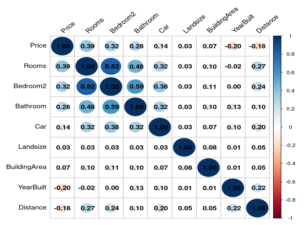
Figure 1: Correlation Analysis (Picture Credit: Original)

Figure 2 suggest histogram associated with the house prices in Melbourne whereby it is observed that the distribution is skewed. In other words, the histogram suggests high volatility in the prices of properties within Melbourne region. In order to rectify this skewness, the price variable is log transformed and the resultant figure is suggested through a histogram in Figure 3. It is observed that the skewness in the price level is normalized or standardized through appropriate transformation of the variable. It further reduces the potential bias in the final estimation of the regression models which indicates accuracy of the research findings.

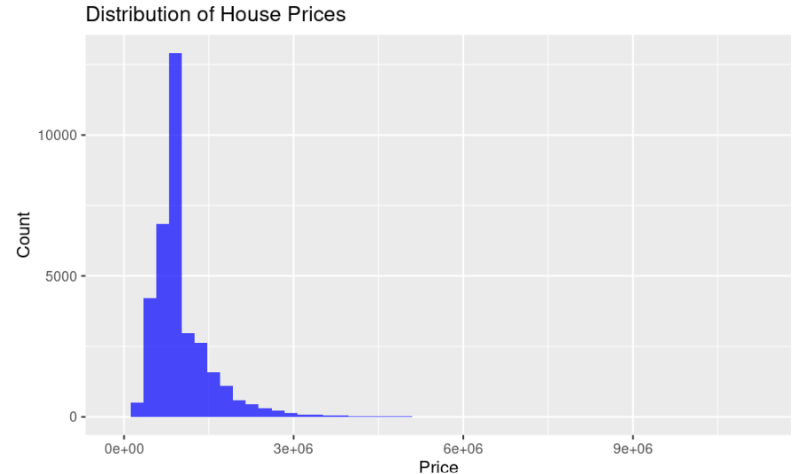
Figure 2: Distribution of house prices (Picture Credit: Original)

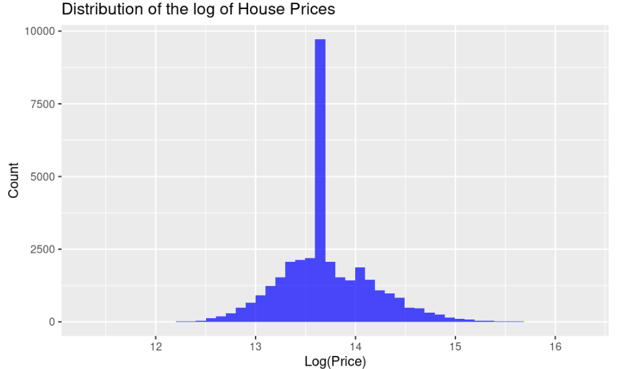
Figure 3: Distribution of house prices: Log transformed (Picture Credit: Original)

Figure 4 suggests that boxplots associated with the price of properties in Melbourne by different number of Rooms. The findings suggest high volatility and outliers in the prices of properties with approximately seven rooms.

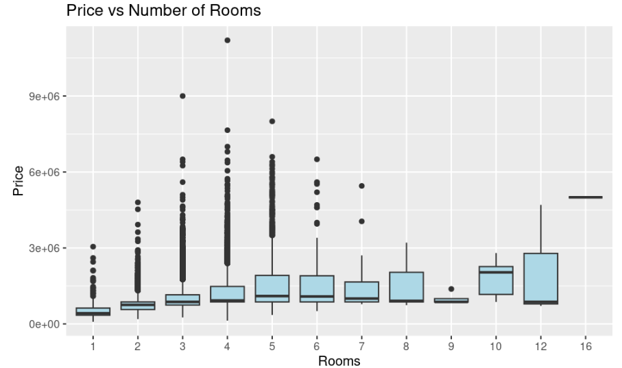
Figure 4: Boxplot of prices by number of rooms (Picture Credit: Original)

Figure 5 shows the relationship between price of the property and the land size of property to understand the association between spatial features of the property and its value. The figure highlights that price and land size are positively related whereby the price of the property increases when the land size increases.

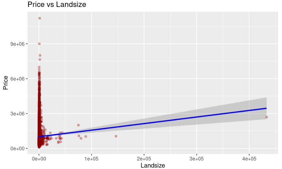
Figure 5: Price and land size (Picture Credit: Original)

Figure 6 suggests the price of the property by different type of property whereby it is observed that significant outliers persist. The findings also suggests that price volatility is more pronounced when the type of the property is house type (h), as compared to townhouse (t) and unit/apartment (u).

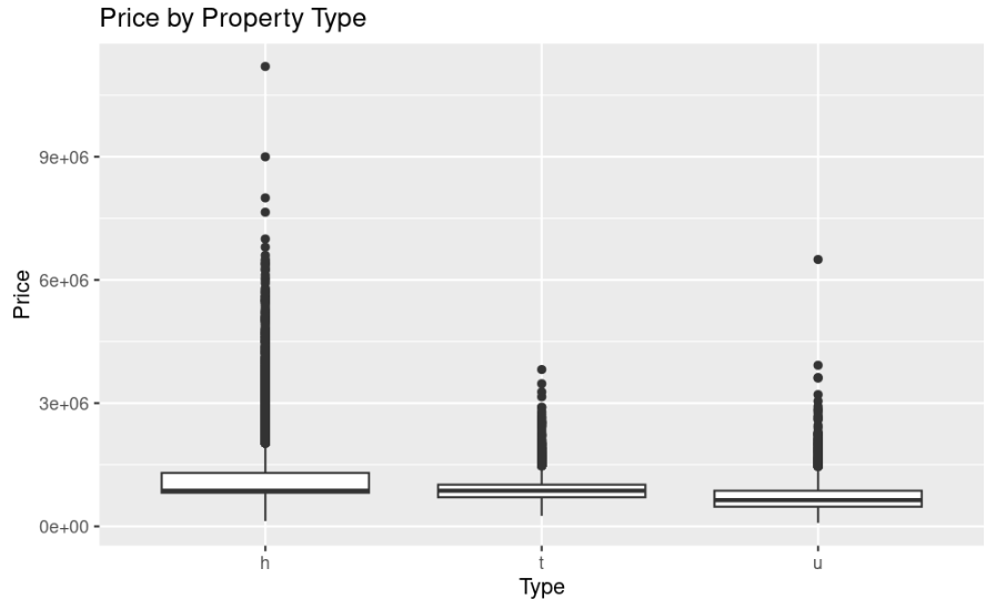
Figure 6: Price by the type of property (Picture Credit: Original)

3.3. Model Selection

In order to select the best model, the current paper computes RMSE and R-square value of each model. The selected predictors comprise type of the property, room, cars, bathroom, land size, building area, year built, distance, and method. Some of the categorical variables like suburbs, regions, and council area are excluded in the final models so that a robust model with distinct qualities is obtained instead of extensively skewed model with only suburbs or region-based information.

Table 4: Accuracy parameters of models

Table 4 highlights the accuracy metrics of each model whereby it is observed that linear and ridge regression model performed considerably better than lasso model, in terms of R-square value and RMSE (root mean square error). R-square value is selected to identify the predictive capacity of the models while RMSE value is considered to determine the prediction accuracy of the models. A model with low RMSE generally indicates less prediction error which is suitable for accurate prediction of house price [10][11]. Linear regression was chosen as the baseline model for its simplicity and interpretability, offering a clear way to understand the relationship between house prices and various property characteristics. This model assumes a linear association between the dependent variable (house price) and independent variables such as the number of rooms, building area, and other attributes. By holding other factors constant, it enables an examination of how each variable affects house prices. The performance of the linear regression model, measured by an R-squared value of 0.3077, indicates that approximately 30.8% of the variation in house prices is explained by the selected features. While this is a reasonable starting point, it also suggests that the model is likely underfitting the data, as nearly 70% of the variability in prices remains unexplained. The RMSE value of 0.855 suggests the average discrepancies in the forecasted house prices by linear regression model.

Besides the baseline model, another variant of regression analysis was use whereby ridge regression model was implemented. The model is suitable when the key factors in the analysis of interest encounters multicollinearity issues or high association between the potential predictors in the model. In case of high multicollinearity, the results from the regression estimates can be considered as spurious in nature which may hamper the credibility of the results. In table 4, it is observed that the R-square and RMSE value of ridge regression model is exactly same as the linear regression which suggests that both models perform relatively same in terms of forecasting the property prices.

Lastly, Lasso regression was introduced due to its capability for feature selection. Unlike Ridge, Lasso can reduce some coefficients to zero, effectively removing less important variables from the model. This can simplify the model and enhance its interpretability without substantially compromising predictive accuracy. However, in this analysis, Lasso regression slightly underperformed compared to the linear and Ridge models, with an R-squared value of 0.3015 and an RMSE of 0.859. The lower R-squared value suggests that Lasso explained slightly less variance in house prices, likely because its penalty zeroed out variables that still contributed marginally to the prediction.

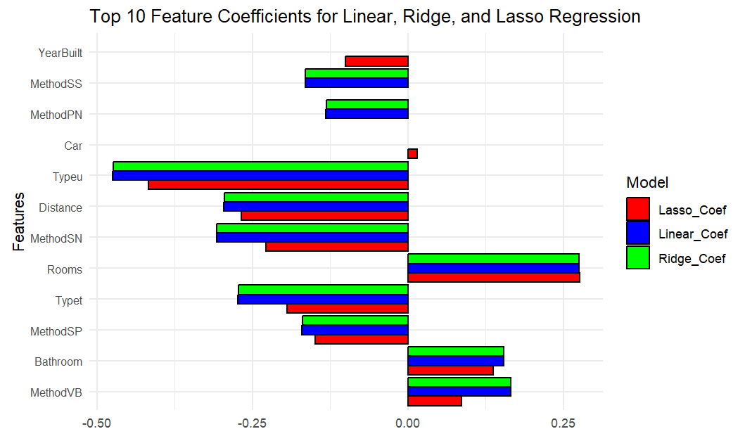
Figure 7: Top 10 features from regression models (Picture Credit: Original)

Figure 7 shows the coefficients for the top ten features influencing Melbourne house prices across Linear, Ridge, and Lasso regression models. Rooms emerges as the most significant predictor, with a positive coefficient indicating that larger homes are valued higher, while Distance from the city centre negatively affects prices, suggesting that properties further away are generally cheaper. The property types Unit/Apartments and Townhouses also show significant negative coefficients, indicating lower values compared to standalone houses. Year Built has a modest positive influence, indicating newer properties are slightly more valuable. Lasso regression notably compresses coefficients, especially for features such as Method SN and Method VB, highlighting its function in feature selection by diminishing the impact of less significant variables.

4. Discussion

The findings from the exploratory data analysis and regression model analysis highlights significant insights regarding Melbourne housing market. Initially, the exploratory analysis reveals key trends and characteristics of the properties, indicating a diverse range of prices and types. The frequency analysis suggests that suburbs like Reservoir, Bentleigh East, and Richmond are the highest demand suburbs for detached family homes. These findings are in line with the contemporary research which highlights the significance of suburbs relevance in property price [7]. In other words, the importance of the suburbs among people can significantly influence the property prices which suggests the diversity of the market.

Standard private sales and auction processes are the most popular sales methods, according to a further assessment that was conducted using frequency analysis. These methodologies are representative of the most common and usual practices that are utilized in the Australian real estate market [3][4]. The widespread use of auctions is indicative of a competitive market in which sellers take advantage of increased demand in order to attain reasonable pricing for their products. Furthermore, the fact that a considerable number of houses are located in the Boroondara City Council and Southern Metropolitan zones suggest that these council areas are the most important locations in terms of the property valuation. The contemporary literature also suggests that the significance of the locations that are close to properties can exert positive externality which in turn increases the overall value of the properties [7]. The findings from analysis also indicate that the most prevalent types of property in Australia are houses (23,980), followed by townhouses and units or flats. This finding is in line with the previous research which suggests that the common preference of house types is the major indicator of property valuation in the region [8]. It indicates that the majority of Australian households prefer to live in one of these types of properties which help property sellers and investors in understanding the preference of the potential buyers.

In terms of the numerical variables, the property price ranges from $85,000 to $11.2 million which indicates that there are both inexpensive housing options and premium houses available in the region. In other words, the extensive price range is also indicative of the wide variety of properties by different affordability factors. With a median price of $870,000, the typical property is within the moderate to high-value range. On the other hand, the fact that the mean price is higher than the median price indicates that luxury listings are having an impact on the average. In addition, the interquartile range that contains a substantial share of transactions is between $695,000 and $1,150,000, which is indicative of a solid housing market for the middle class. Due to the fact that the correlation analysis reveals the existence of potential multicollinearity problems between the number of bedrooms and other variables, it is necessary to exclude Bedroom 2 from the further modelling. The importance of this step cannot be overstated when it comes to assuring the dependability of regression estimates and preventing skewed interpretations of the connection between property attributes and pricing. The original skewness that was noticed in the data distribution has been successfully mitigated by the use of log transformation of the price variable, which has resulted in an improvement in the accuracy of the regression models. The histogram comparisons that were performed before and after the modification demonstrate a dataset that has been more normalized, which enables improved predictive modelling. The examination of the boxplot shows further information about the volatility and the presence of outliers, particularly in houses that have seven rooms. This indicates that there are distinct market niches that require further investigation, also highlighted in the contemporary research.

In order to implement the selected models, the current papers select certain numerical variables and categorical variables (like types and methods). The primary goal of the paper is to develop a robust model which captures distinct information regarding the factors affecting property prices in Melbourne. The positive association that is anticipated in real estate markets is confirmed by the relationship between price and land size, which is illustrated in the analysis. Generally speaking, greater land areas attract higher prices. According to Soltani et al. [13], this finding is consistent with broader trends in housing markets, where the size of the land is a significant factor in determining the value of a property. The linear regression model and the ridge regression model both displayed equivalent efficacy in terms of model performance. Both models explained around 30.8% of the variation in housing prices. However, despite the fact that this level of explanatory power provides a good framework for further investigation, it also shows that there are other elements that are not included in the model that may contribute considerably to price. Given the complexity of the housing market, it is advisable to use linear regression as the baseline model because of its simplicity and interpretability. This decision was made because linear regression is easy to understand. The feature selection capabilities of lasso regression are particularly important since they simplify the model by eliminating predictors that are not as significant. On the other hand, the fact that it performed somewhat worse than expected in this analysis suggests that it strikes a cautious compromise between simplicity and predictive capability. The coefficients that were produced from the various models provide more evidence that the conclusions are accurate. The room count was shown to be the most influential predictor, followed by the kind of property and the distance from the city center.

The findings from the analysis will aid investors, potential property buyers, sellers, and government authorities in Australia. For example, the information pertaining to price volatility can assist investors in understanding the nature of the market. The demand for certain properties, based on specific features, can help property dealers and sellers in understanding the market demand. By leveraging these insights, the sellers can better position themselves in the market and target customers according to their needs. Furthermore, it will allow property owners to maintain their properties accordingly so that their overall value can increase. For instance, homeowners can focus on enhancing key attributes such as energy efficiency, aesthetics, and the quality of amenities, which can lead to an increase in property values over time. Additionally, property owners can utilize the insights to make informed decisions about renovations or upgrades that align with current market preferences, thus maximizing their investment returns.

The government and other housing regulatory authorities can leverage the findings to understand the demand and supply within the real estate market. By analysing trends, policymakers can identify areas where intervention may be necessary to stabilize the market or address affordability issues. In the case of extreme prices, the authorities can implement necessary regulations to avoid the violation of property purchase and selling rules and disruptions in the market due to extremely high prices. This proactive approach can prevent housing bubbles and ensure that the market remains accessible to a broader range of buyers, thereby promoting housing stability. Additionally, the findings can be useful in guiding urban planning and development strategies to the government and planning authorities in a country. By understanding the factors that influence property prices, it will help city planners make informed decisions regarding zoning, infrastructure development, and public transportation projects. By aligning these initiatives with the identified market trends, authorities can enhance the accessibility and the overall growth in the property value within Melbourne region.

Overall, the research findings positively contribute to the existing pool of literature by highlighting the significance of insights for different types of stakeholders while using robust modeling approaches. These insights not only enhance the understanding of the current housing landscape but also serve as a foundation for future research. This can lead to more nuanced studies that explore additional variables, demographic shifts, and the long-term effects of economic conditions on the housing market. By continuing to build upon this research, stakeholders can better navigate the complexities of the real estate market in Australia, ultimately fostering a more informed and resilient housing environment.

5. Conclusion

To sum up, the current research paper aims to predict house prices in Melbourne area while targeting the physical characteristics of the properties in the region. The primary objectives of the analysis are to identify the most critical factors which influence property price in the region. The second aim of the analysis is to identify a robust regression model which help forecast the prices with the least error. The paper initially discusses the rationale of the study and the findings from the contemporary literature whereby it was observed that most of the studies include macroeconomic indicators like GDP, employment rate, interest rate, and current investment levels to determine the price of the properties. By considering the findings from the contemporary literature, the current research aims to identify the most important factors affecting the house prices in Melbourne and the most robust regression model which help predict accurate house prices in the region. The findings from the regression estimates reveal that ridge and linear regression models are the most promising and the robust models in terms of property prices. The RMSE and R-squared value of each model remained same as compared to the lasso model. The feature selection also suggested that type of the property, year of built, distance, car, room, and bathroom are some of the most essential factors which affects the property prices in the region. The overall analysis fulfills the two central objectives of the paper: to identify the most significant predictors of property prices and to identify the most robust model for prediction. The practical implications of the findings are considerably advance and comprehensive.

Besides extensive strengths of the analysis, the main limitations of the analysis are lack of generalizability because the results are only relevant for Melbourne region. While housing trends in a given locale stem from its distinctive makeup, the results here may lack reach. Comparative looks across other Australian metros could help uncover which influences withstand borders and which fade, bringing light to pricing propensities' true scale. Future analyses may broaden insight by balancing metro-specific aspects with intercity examinations, teasing out recurrent patterns beneath geographic variances. Another limitation of the analysis is potential exclusion bias because certain categorical variables related to suburbs, regions, and council areas are excluded. The rationale of removing these variables was to reduce excessive skewness in the research findings so that distinct critical factors can be included in the analysis. Furthermore, the presence of outliers, particularly in high-value properties, can distort the overall findings of the analysis. While the study implemented log transformation to mitigate skewness in the price variable, the impact of outliers still necessitates further scrutiny. Future research should explore advanced statistical techniques to better handle outliers, such as robust regression methods, which can provide more reliable estimates when dealing with skewed data.

In order to enhance the quality of the analysis, the future research should include a wide range of variables which may include both macroeconomic factors and physical characteristics. While the analysis has identified key physical characteristics that influence property prices, the focus on these specific variables may overlook other important factors. For instance, macroeconomic indicators such as interest rates, inflation, and employment rates are known to have a substantial impact on housing demand and prices. Similarly, social factors, such as demographic shifts and changes in consumer preferences, are vital in understanding housing trends. Future research should aim to include a more comprehensive set of variables to provide a holistic view of the factors influencing property prices in Melbourne. While extending upon the analysis from previous section, future studies can consider other countries or regions to understand if factors vary across areas or regions in terms of property prices. By investigating the effects of government policies, such as housing subsidies, zoning regulations, and taxation, on property values can yield critical insights into the efficacy of interventions designed to enhance housing affordability. Understanding how these policies interact with market forces can help inform better policy decisions in the future. Future research should also delve into consumer behavior to understand the preferences and motivations of home-buyers better. By utilizing qualitative methods to complement quantitative analysis, researchers can gain insights into the factors influencing buyer decisions, such as lifestyle preferences, community amenities, and proximity to schools and workplaces.

References

[1]. Liu, G. (2022). Research on prediction and analysis of real estate market based on the multiple linear regression model. *Scientific Programming, 1–8. https://doi.org/10.1155/2022/5750354
[2]. Gurran, N., & Phibbs, P. (2013). Housing supply and urban planning reform: The recent Australian experience, 2003–2012. *International Journal of Housing Policy, 13*(4), 381–407. https://doi.org/10.1080/14616718.2013.840110
[3]. Phan, T. D. (2018). Housing price prediction using machine learning algorithms: The case of Melbourne city, Australia. In *2018 International Conference on Machine Learning and Data Engineering (iCMLDE)* (pp. 35–42). https://doi.org/10.1109/iCMLDE.2018.00017
[4]. Mouna, L. E., Silkan, H., Haynf, Y., Nann, M. F., & Tekouabou, S. C. K. (2023). A comparative study of urban house price prediction using machine learning algorithms. *E3S Web of Conferences, 418*, 03001. https://doi.org/10.1051/e3sconf/202341803001
[5]. Sari, R., Ewing, B. T., & Aydin, B. (2007). Macroeconomic variables and the housing market in Turkey. *Emerging Markets Finance and Trade, 43*(5), 5–19. https://doi.org/10.2753/REE1540-496X430501
[6]. Rosen, S. (1974). Hedonic prices and implicit markets: Product differentiation in pure competition. *Journal of Political Economy, 82*(1), 34–55. http://www.jstor.org/stable/1830899
[7]. Malpezzi, S. (2002). Hedonic pricing models: A selective and applied review. In T. O’Sullivan & K. Gibb (Eds.), *Housing economics and public policy* (1st ed., pp. 67–89). Wiley. https://doi.org/10.1002/9780470690680.ch5
[8]. Pawson, H., Milligan, V., & Yates, J. (2020). Housing policy in Australia: A reform agenda. In *Housing policy in Australia: A case for system reform* (pp. 339–358). Springer Nature. https://doi.org/10.1007/978-981-15-0780-9_10
[9]. Rey-Blanco, D., Zofío, J. L., & González-Arias, J. (2024). Improving hedonic housing price models by integrating optimal accessibility indices into regression and random forest analyses. *Expert Systems with Applications, 235*, 121059. https://doi.org/10.1016/j.eswa.2023.121059
[10]. Yoo, S., Im, J., & Wagner, J. E. (2012). Variable selection for hedonic model using machine learning approaches: A case study in Onondaga County, NY. *Landscape and Urban Planning, 107*(3), 293–306. https://doi.org/10.1016/j.landurbplan.2012.06.009
[11]. Yazdani, M. (2021). House price determinants and market segmentation in Boulder, Colorado: A hedonic price approach. *arXiv*. https://doi.org/10.48550/arXiv.2108.02442
[12]. Nguyen, M.-L. T. (2020). The hedonic pricing model applied to the housing market. *International Journal of Economics and Business Administration, 8*(3), 416–428. https://ijeba.com/journal/526
[13]. Soltani, A., Heydari, M., Aghaei, F., & Pettit, C. J. (2022). Housing price prediction incorporating spatio-temporal dependency into machine learning algorithms. *Cities, 131*, 103941. https://doi.org/10.1016/j.cities.2022.103941
[14]. Kaggle. (2024). Melbourne housing market. https://www.kaggle.com/datasets/anthonypino/melbourne-housing-market
[15]. Deshpande, A., & Kumar, M. (2018). *Artificial intelligence for big data: Complete guide to automating big data solutions using artificial intelligence techniques*. Packt Publishing Limited.
[16]. Refaat, M. (2007). *Data preparation for data mining using SAS*. Morgan Kaufmann Publishers.
[17]. Weinberg, S. L., Harel, D., & Abramowitz, S. K. (2023). *Statistics using R: An integrative approach* (2nd ed.). Cambridge University Press.
Cite this article
Zhao,X. (2024). Analysing Melbourne's Property Market Dynamics: A Hedonic Price Prediction Approach Using Real Estate Data. Advances in Economics, Management and Political Sciences,143,48-64.
Data availability
The datasets used and/or analyzed during the current study will be available from the authors upon reasonable request.
Disclaimer/Publisher's Note
The statements, opinions and data contained in all publications are solely those of the individual author(s) and contributor(s) and not of EWA Publishing and/or the editor(s). EWA Publishing and/or the editor(s) disclaim responsibility for any injury to people or property resulting from any ideas, methods, instructions or products referred to in the content.
About volume
Volume title: Proceedings of ICFTBA 2024 Workshop: Finance's Role in the Just Transition
© 2024 by the author(s). Licensee EWA Publishing, Oxford, UK. This article is an open access article distributed under the terms and
conditions of the Creative Commons Attribution (CC BY) license. Authors who
publish this series agree to the following terms:
1. Authors retain copyright and grant the series right of first publication with the work simultaneously licensed under a Creative Commons
Attribution License that allows others to share the work with an acknowledgment of the work's authorship and initial publication in this
series.
2. Authors are able to enter into separate, additional contractual arrangements for the non-exclusive distribution of the series's published
version of the work (e.g., post it to an institutional repository or publish it in a book), with an acknowledgment of its initial
publication in this series.
3. Authors are permitted and encouraged to post their work online (e.g., in institutional repositories or on their website) prior to and
during the submission process, as it can lead to productive exchanges, as well as earlier and greater citation of published work (See
Open access policy for details).